IT training introduction to pattern recognition and machine learning murty devi 2014 09 30
Bạn đang xem bản rút gọn của tài liệu. Xem và tải ngay bản đầy đủ của tài liệu tại đây (2.29 MB, 402 trang )
8037_9789814335454_tp.indd 1
26/2/15 12:15 pm
IISc Lecture Notes Series
ISSN: 2010-2402
Editor-in-Chief: Gadadhar Misra
Editors: Chandrashekar S Jog
Joy Kuri
K L Sebastian
Diptiman Sen
Sandhya Visweswariah
Published:
Vol. 1: Introduction to Algebraic Geometry and Commutative Algebra
by Dilip P Patil & Uwe Storch
Vol. 2: Schwarz’s Lemma from a Differential Geometric Veiwpoint
by Kang-Tae Kim & Hanjin Lee
Vol. 3: Noise and Vibration Control
by M L Munjal
Vol. 4: Game Theory and Mechanism Design
by Y Narahari
Vol. 5 Introduction to Pattern Recognition and Machine Learning
by M. Narasimha Murty & V. Susheela Devi
Dipa - Introduction to pattern recognition.indd 1
10/4/2015 1:29:09 PM
World Scientific
8037_9789814335454_tp.indd 2
26/2/15 12:15 pm
Published by
World Scientific Publishing Co. Pte. Ltd.
5 Toh Tuck Link, Singapore 596224
USA office: 27 Warren Street, Suite 401-402, Hackensack, NJ 07601
UK office: 57 Shelton Street, Covent Garden, London WC2H 9HE
Library of Congress Cataloging-in-Publication Data
Murty, M. Narasimha.
Introduction to pattern recognition and machine learning / by M Narasimha Murty &
V Susheela Devi (Indian Institute of Science, India).
pages cm. -- (IISc lecture notes series, 2010–2402 ; vol. 5)
ISBN 978-9814335454
1. Pattern recognition systems. 2. Machine learning. I. Devi, V. Susheela. II. Title.
TK7882.P3M87 2015
006.4--dc23
2014044796
British Library Cataloguing-in-Publication Data
A catalogue record for this book is available from the British Library.
Copyright © 2015 by World Scientific Publishing Co. Pte. Ltd.
All rights reserved. This book, or parts thereof, may not be reproduced in any form or by any means,
electronic or mechanical, including photocopying, recording or any information storage and retrieval
system now known or to be invented, without written permission from the publisher.
For photocopying of material in this volume, please pay a copying fee through the Copyright Clearance
Center, Inc., 222 Rosewood Drive, Danvers, MA 01923, USA. In this case permission to photocopy
is not required from the publisher.
In-house Editors: Chandra Nugraha/Dipasri Sardar
Typeset by Stallion Press
Email:
Printed in Singapore
Dipa - Introduction to pattern recognition.indd 3
10/4/2015 1:29:09 PM
Series Preface
World Scientific Publishing Company - Indian Institute of Science Collaboration
IISc Press and WSPC are co-publishing books authored by world renowned scientists and engineers. This collaboration, started in 2008 during IISc’s centenary
year under a Memorandum of Understanding between IISc and WSPC, has resulted
in the establishment of three Series: IISc Centenary Lectures Series (ICLS), IISc
Research Monographs Series (IRMS), and IISc Lecture Notes Series (ILNS).
This pioneering collaboration will contribute significantly in disseminating current
Indian scientific advancement worldwide.
The “IISc Centenary Lectures Series” will comprise lectures by designated
Centenary Lecturers - eminent teachers and researchers from all over the world.
The “IISc Research Monographs Series” will comprise state-of-the-art monographs written by experts in specific areas. They will include, but not limited to,
the authors’ own research work.
The “IISc Lecture Notes Series” will consist of books that are reasonably selfcontained and can be used either as textbooks or for self-study at the postgraduate
level in science and engineering. The books will be based on material that has been
class-tested for most part.
Editorial Board for the IISc Lecture Notes Series (ILNS):
Gadadhar Misra, Editor-in-Chief ()
Chandrashekar S Jog ()
Joy Kuri ()
K L Sebastian ()
Diptiman Sen ()
Sandhya Visweswariah ()
Dipa - Introduction to pattern recognition.indd 2
10/4/2015 1:29:09 PM
May 2, 2013
14:6
BC: 8831 - Probability and Statistical Theory
This page intentionally left blank
PST˙ws
April 8, 2015
13:2
Introduction to Pattern Recognition and Machine Learning - 9in x 6in
b1904-fm
page vii
Table of Contents
About the Authors
xiii
Preface
1.
Introduction
1.
2.
3.
2.
xv
1
Classifiers: An Introduction . . . . . . . . . . . . . .
An Introduction to Clustering . . . . . . . . . . . . .
Machine Learning . . . . . . . . . . . . . . . . . . .
Types of Data
1.
2.
3.
4.
5
14
25
37
Features and Patterns . . . . . . . . . . . .
Domain of a Variable . . . . . . . . . . . .
Types of Features . . . . . . . . . . . . . .
3.1. Nominal data . . . . . . . . . . . . .
3.2. Ordinal data . . . . . . . . . . . . . .
3.3. Interval-valued variables . . . . . . .
3.4. Ratio variables . . . . . . . . . . . . .
3.5. Spatio-temporal data . . . . . . . . .
Proximity measures . . . . . . . . . . . . .
4.1. Fractional norms . . . . . . . . . . .
4.2. Are metrics essential? . . . . . . . . .
4.3. Similarity between vectors . . . . . .
4.4. Proximity between spatial patterns .
4.5. Proximity between temporal patterns
vii
.
.
.
.
.
.
.
.
.
.
.
.
.
.
.
.
.
.
.
.
.
.
.
.
.
.
.
.
.
.
.
.
.
.
.
.
.
.
.
.
.
.
.
.
.
.
.
.
.
.
.
.
.
.
.
.
.
.
.
.
.
.
.
.
.
.
.
.
.
.
37
39
41
41
45
48
49
49
50
56
57
59
61
62
April 8, 2015
13:2
Introduction to Pattern Recognition and Machine Learning - 9in x 6in
viii
page viii
Table of Contents
4.6.
4.7.
4.8.
4.9.
3.
b1904-fm
Mean dissimilarity . . . . . . . .
Peak dissimilarity . . . . . . . .
Correlation coefficient . . . . . .
Dynamic Time Warping (DTW)
. . . . .
. . . . .
. . . . .
distance
.
.
.
.
.
.
.
.
.
.
.
.
Feature Extraction and Feature Selection
1.
2.
3.
4.
5.
6.
7.
8.
9.
10.
11.
12.
13.
Types of Feature Selection . . . . . . . . . . . . . .
Mutual Information (MI) for Feature Selection . .
Chi-square Statistic . . . . . . . . . . . . . . . . .
Goodman–Kruskal Measure . . . . . . . . . . . . .
Laplacian Score . . . . . . . . . . . . . . . . . . . .
Singular Value Decomposition (SVD) . . . . . . .
Non-negative Matrix Factorization (NMF) . . . . .
Random Projections (RPs) for Feature
Extraction . . . . . . . . . . . . . . . . . . . . . .
8.1. Advantages of random projections . . . . . .
Locality Sensitive Hashing (LSH) . . . . . . . . . .
Class Separability . . . . . . . . . . . . . . . . . .
Genetic and Evolutionary Algorithms . . . . . . .
11.1. Hybrid GA for feature selection . . . . . . .
Ranking for Feature Selection . . . . . . . . . . . .
12.1. Feature selection based on an optimization
formulation . . . . . . . . . . . . . . . . . . .
12.2. Feature ranking using F-score . . . . . . . .
12.3. Feature ranking using linear support vector
machine (SVM) weight vector . . . . . . . .
12.4. Ensemble feature ranking . . . . . . . . . . .
12.5. Feature ranking using number
of label changes . . . . . . . . . . . . . . . .
Feature Selection for Time Series Data . . . . . . .
13.1. Piecewise aggregate approximation . . . . .
13.2. Spectral decomposition . . . . . . . . . . . .
13.3. Wavelet decomposition . . . . . . . . . . . .
13.4. Singular Value Decomposition (SVD) . . . .
13.5. Common principal component loading based
variable subset selection (CLeVer) . . . . . .
63
63
64
64
75
.
.
.
.
.
.
.
76
78
79
81
81
83
84
.
.
.
.
.
.
.
86
88
88
90
91
92
96
.
.
97
99
.
.
100
101
.
.
.
.
.
.
103
103
103
104
104
104
.
104
April 8, 2015
13:2
Introduction to Pattern Recognition and Machine Learning - 9in x 6in
b1904-fm
Table of Contents
4.
5.
ix
Bayesian Learning
1.
2.
3.
4.
5.
6.
Document Classification . . . . . . . . . . . .
Naive Bayes Classifier . . . . . . . . . . . . .
Frequency-Based Estimation of Probabilities
Posterior Probability . . . . . . . . . . . . . .
Density Estimation . . . . . . . . . . . . . . .
Conjugate Priors . . . . . . . . . . . . . . . .
111
.
.
.
.
.
.
.
.
.
.
.
.
.
.
.
.
.
.
.
.
.
.
.
.
Classification
1.
2.
3.
4.
5.
6.
7.
Classification Without Learning . . . . . . .
Classification in High-Dimensional Spaces . .
2.1. Fractional distance metrics . . . . . . .
2.2. Shrinkage–divergence proximity (SDP)
Random Forests . . . . . . . . . . . . . . . .
3.1. Fuzzy random forests . . . . . . . . . .
Linear Support Vector Machine (SVM) . . .
4.1. SVM–kNN . . . . . . . . . . . . . . . .
4.2. Adaptation of cutting plane algorithm
4.3. Nystrom approximated SVM . . . . . .
Logistic Regression . . . . . . . . . . . . . . .
Semi-supervised Classification . . . . . . . . .
6.1. Using clustering algorithms . . . . . . .
6.2. Using generative models . . . . . . . .
6.3. Using low density separation . . . . . .
6.4. Using graph-based methods . . . . . .
6.5. Using co-training methods . . . . . . .
6.6. Using self-training methods . . . . . . .
6.7. SVM for semi-supervised classification
6.8. Random forests for semi-supervised
classification . . . . . . . . . . . . . . .
Classification of Time-Series Data . . . . . .
7.1. Distance-based classification . . . . . .
7.2. Feature-based classification . . . . . . .
7.3. Model-based classification . . . . . . .
page ix
111
113
115
117
119
126
135
.
.
.
.
.
.
.
.
.
.
.
.
.
.
.
.
.
.
.
.
.
.
.
.
.
.
.
.
.
.
.
.
.
.
.
.
.
.
.
.
.
.
.
.
.
.
.
.
.
.
.
.
.
.
.
.
.
.
.
.
.
.
.
.
.
.
.
.
.
.
.
.
.
.
.
.
135
139
141
143
144
148
150
153
154
155
156
159
160
160
161
162
164
165
166
.
.
.
.
.
.
.
.
.
.
.
.
.
.
.
.
.
.
.
.
166
167
168
169
170
April 8, 2015
13:2
Introduction to Pattern Recognition and Machine Learning - 9in x 6in
x
6.
Table of Contents
Classification using Soft Computing Techniques
1.
2.
3.
4.
5.
6.
7.
b1904-fm
Introduction . . . . . . . . . . . . . . . . . . .
Fuzzy Classification . . . . . . . . . . . . . . .
2.1. Fuzzy k-nearest neighbor algorithm . . .
Rough Classification . . . . . . . . . . . . . . .
3.1. Rough set attribute reduction . . . . . .
3.2. Generating decision rules . . . . . . . . .
GAs . . . . . . . . . . . . . . . . . . . . . . . .
4.1. Weighting of attributes using GA . . . .
4.2. Binary pattern classification using GA .
4.3. Rule-based classification using GAs . . .
4.4. Time series classification . . . . . . . . .
4.5. Using generalized Choquet integral with
signed fuzzy measure for classification
using GAs . . . . . . . . . . . . . . . . .
4.6. Decision tree induction using
Evolutionary algorithms . . . . . . . . .
Neural Networks for Classification . . . . . . .
5.1. Multi-layer feed forward network
with backpropagation . . . . . . . . . . .
5.2. Training a feedforward neural network
using GAs . . . . . . . . . . . . . . . . .
Multi-label Classification . . . . . . . . . . . .
6.1. Multi-label kNN (mL-kNN) . . . . . . .
6.2. Probabilistic classifier chains (PCC) . . .
6.3. Binary relevance (BR) . . . . . . . . . .
6.4. Using label powersets (LP) . . . . . . . .
6.5. Neural networks for Multi-label
classification . . . . . . . . . . . . . . . .
6.6. Evaluation of multi-label classification .
.
.
.
.
.
.
.
.
.
.
.
.
.
.
.
.
.
.
.
.
.
.
177
.
.
.
.
.
.
.
.
.
.
.
177
178
179
179
180
181
182
182
184
185
187
. . .
187
. . .
. . .
191
195
. . .
197
.
.
.
.
.
.
.
.
.
.
.
.
199
202
203
204
205
205
. . .
. . .
206
209
.
.
.
.
.
.
Data Clustering
215
1.
2.
215
218
219
Number of Partitions . . . . . . . . . . . . . . . . .
Clustering Algorithms . . . . . . . . . . . . . . . . .
2.1. K-means algorithm . . . . . . . . . . . . . . .
page x
April 8, 2015
13:2
Introduction to Pattern Recognition and Machine Learning - 9in x 6in
b1904-fm
Table of Contents
2.2.
2.3.
3.
4.
5.
8.
Leader algorithm . . . . . . . . . . .
BIRCH: Balanced Iterative Reducing
and Clustering using Hierarchies . . .
2.4. Clustering based on graphs . . . . . .
Why Clustering? . . . . . . . . . . . . . . .
3.1. Data compression . . . . . . . . . . .
3.2. Outlier detection . . . . . . . . . . .
3.3. Pattern synthesis . . . . . . . . . . .
Clustering Labeled Data . . . . . . . . . . .
4.1. Clustering for classification . . . . . .
4.2. Knowledge-based clustering . . . . .
Combination of Clusterings . . . . . . . . .
xi
. . . . .
223
.
.
.
.
.
.
.
.
.
.
225
230
241
241
242
243
246
246
250
255
.
.
.
.
.
.
.
.
.
.
.
.
.
.
.
.
.
.
.
.
.
.
.
.
.
.
.
.
.
.
.
.
.
.
.
.
.
.
.
.
Soft Clustering
1.
2.
3.
4.
5.
6.
7.
page xi
Soft Clustering Paradigms . . . . . . . . . . .
Fuzzy Clustering . . . . . . . . . . . . . . . .
2.1. Fuzzy K-means algorithm . . . . . . .
Rough Clustering . . . . . . . . . . . . . . . .
3.1. Rough K-means algorithm . . . . . . .
Clustering Based on Evolutionary Algorithms
Clustering Based on Neural Networks . . . .
Statistical Clustering . . . . . . . . . . . . . .
6.1. OKM algorithm . . . . . . . . . . . . .
6.2. EM-based clustering . . . . . . . . . . .
Topic Models . . . . . . . . . . . . . . . . . .
7.1. Matrix factorization-based methods . .
7.2. Divide-and-conquer approach . . . . .
7.3. Latent Semantic Analysis (LSA) . . . .
7.4. SVD and PCA . . . . . . . . . . . . . .
7.5. Probabilistic Latent Semantic Analysis
(PLSA) . . . . . . . . . . . . . . . . . .
7.6. Non-negative Matrix Factorization
(NMF) . . . . . . . . . . . . . . . . . .
7.7. LDA . . . . . . . . . . . . . . . . . . .
7.8. Concept and topic . . . . . . . . . . . .
263
.
.
.
.
.
.
.
.
.
.
.
.
.
.
.
.
.
.
.
.
.
.
.
.
.
.
.
.
.
.
.
.
.
.
.
.
.
.
.
.
.
.
.
.
.
.
.
.
.
.
.
.
.
.
.
.
.
.
.
.
264
266
267
269
271
272
281
282
283
285
293
295
296
299
302
. . . .
307
. . . .
. . . .
. . . .
310
311
316
April 8, 2015
13:2
xii
9.
Introduction to Pattern Recognition and Machine Learning - 9in x 6in
b1904-fm
Table of Contents
Application — Social and Information Networks
1.
2.
3.
4.
5.
6.
7.
Index
Introduction . . . . . . . . . . . . . . . . . . .
Patterns in Graphs . . . . . . . . . . . . . . . .
Identification of Communities in Networks . . .
3.1. Graph partitioning . . . . . . . . . . . .
3.2. Spectral clustering . . . . . . . . . . . . .
3.3. Linkage-based clustering . . . . . . . . .
3.4. Hierarchical clustering . . . . . . . . . .
3.5. Modularity optimization for partitioning
graphs . . . . . . . . . . . . . . . . . . .
Link Prediction . . . . . . . . . . . . . . . . . .
4.1. Proximity functions . . . . . . . . . . . .
Information Diffusion . . . . . . . . . . . . . .
5.1. Graph-based approaches . . . . . . . . .
5.2. Non-graph approaches . . . . . . . . . .
Identifying Specific Nodes in a Social Network
Topic Models . . . . . . . . . . . . . . . . . . .
7.1. Probabilistic latent semantic analysis
(pLSA) . . . . . . . . . . . . . . . . . . .
7.2. Latent dirichlet allocation (LDA) . . . .
7.3. Author–topic model . . . . . . . . . . . .
321
.
.
.
.
.
.
.
.
.
.
.
.
.
.
.
.
.
.
.
.
.
321
322
326
328
329
331
331
.
.
.
.
.
.
.
.
.
.
.
.
.
.
.
.
.
.
.
.
.
.
.
.
333
340
341
347
348
349
353
355
. . .
. . .
. . .
355
357
359
365
page xii
April 8, 2015
13:2
Introduction to Pattern Recognition and Machine Learning - 9in x 6in
b1904-fm
About the Authors
Professor M. Narasimha Murty completed his B.E., M.E., and
Ph.D. at the Indian Institute of Science (IISc), Bangalore. He joined
IISc as an Assistant Professor in 1984. He became a professor in 1996
and currently he is the Dean, Engineering Faculty at IISc. He has
guided more than 20 doctoral students and several masters students
over the past 30 years at IISc; most of these students have worked in
the areas of Pattern Recognition, Machine Learning, and Data Mining. A paper co-authored by him on Pattern Clustering has around
9600 citations as reported by Google scholar. A team led by him
had won the KDD Cup on the citation prediction task organized by
the Cornell University in 2003. He is elected as a fellow of both the
Indian National Academy of Engineering and the National Academy
of Sciences.
Dr. V. Susheela Devi completed her PhD at the Indian Institute
of Science in 2000. Since then she has worked as a faculty in the
Department of Computer Science and Automation at the Indian
Institute of Science. She works in the areas of Pattern Recognition, Data Mining, Machine Learning, and Soft Computing. She has
taught the courses Data Mining, Pattern Recognition, Data Structures and Algorithms, Computational Methods of Optimization and
Artificial Intelligence. She has a number of papers in international
conferences and journals.
xiii
page xiii
May 2, 2013
14:6
BC: 8831 - Probability and Statistical Theory
This page intentionally left blank
PST˙ws
April 8, 2015
13:2
Introduction to Pattern Recognition and Machine Learning - 9in x 6in
b1904-fm
Preface
Pattern recognition (PR) is a classical area and some of the important
topics covered in the books on PR include representation of patterns,
classification, and clustering. There are different paradigms for pattern recognition including the statistical and structural paradigms.
The structural or linguistic paradigm has been studied in the early
days using formal language tools. Logic and automata have been
used in this context. In linguistic PR, patterns could be represented
as sentences in a logic; here, each pattern is represented using a set
of primitives or sub-patterns and a set of operators. Further, a class
of patterns is viewed as being generated using a grammar; in other
words, a grammar is used to generate a collection of sentences or
strings where each string corresponds to a pattern. So, the classification model is learnt using some grammatical inference procedure;
the collection of sentences corresponding to the patterns in the class
are used to learn the grammar. A major problem with the linguistic
approach is that it is suited to dealing with structured patterns and
the models learnt cannot tolerate noise.
On the contrary the statistical paradigm has gained a lot of
momentum in the past three to four decades. Here, patterns are
viewed as vectors in a multi-dimensional space and some of the
optimal classifiers are based on Bayes rule. Vectors corresponding
to patterns in a class are viewed as being generated by the underlying probability density function; Bayes rule helps in converting the
prior probabilities of the classes into posterior probabilities using the
xv
page xv
April 8, 2015
xvi
13:2
Introduction to Pattern Recognition and Machine Learning - 9in x 6in
b1904-fm
Preface
likelihood values corresponding to the patterns given in each class.
So, estimation schemes are used to obtain the probability density
function of a class using the vectors corresponding to patterns in the
class. There are several other classifiers that work with vector representation of patterns. We deal with statistical pattern recognition in
this book.
Some of the simplest classification and clustering algorithms are
based on matching or similarity between vectors. Typically, two patterns are similar if the distance between the corresponding vectors is
lesser; Euclidean distance is popularly used. Well-known algorithms
including the nearest neighbor classifier (NNC), K-nearest neighbor
classifier (KNNC), and the K-Means Clustering algorithm are based
on such distance computations. However, it is well understood in the
literature that distance between two vectors may not be meaningful if the vectors are in large-dimensional spaces which is the case in
several state-of-the-art application areas; this is because the distance
between a vector and its nearest neighbor can tend to the distance
between the pattern and its farthest neighbor as the dimensionality
increases. This prompts the need to reduce the dimensionality of the
vectors. We deal with the representation of patterns, different types
of components of vectors and the associated similarity measures in
Chapters 2 and 3.
Machine learning (ML) also has been around for a while;
early efforts have concentrated on logic or formal language-based
approaches. Bayesian methods have gained prominence in ML in
the recent decade; they have been applied in both classification and
clustering. Some of the simple and effective classification schemes
are based on simplification of the Bayes classifier using some acceptable assumptions. Bayes classifier and its simplified version called
the Naive Bayes classifier are discussed in Chapter 4. Traditionally there has been a contest between the frequentist approaches
like the Maximum-likelihood approach and the Bayesian approach.
In maximum-likelihood approaches the underlying density is estimated based on the assumption that the unknown parameters are
deterministic; on the other hand the Bayesian schemes assume that
the parameters characterizing the density are unknown random variables. In order to make the estimation schemes simpler, the notion
page xvi
April 8, 2015
13:2
Introduction to Pattern Recognition and Machine Learning - 9in x 6in
Preface
b1904-fm
page xvii
xvii
of conjugate pair is exploited in the Bayesian methods. If for a given
prior density, the density of a class of patterns is such that, the posterior has the same density function as the prior, then the prior and
the class density form a conjugate prior. One of the most exploited in
the context of clustering are the Dirichlet prior and the Multinomial
class density which form a conjugate pair. For a variety of such conjugate pairs it is possible to show that when the datasets are large
in size, there is no difference between the maximum-likelihood and
the Bayesian estimates. So, it is important to examine the role of
Bayesian methods in Big Data applications.
Some of the most popular classifiers are based on support vector
machines (SVMs), boosting, and Random Forest. These are discussed
in Chapter 5 which deals with classification. In large-scale applications like text classification where the dimensionality is large, linear
SVMs and Random Forest-based classifiers are popularly used. These
classifiers are well understood in terms of their theoretical properties.
There are several applications where each pattern belongs to more
than one class; soft classification schemes are required to deal with
such applications. We discuss soft classification schemes in Chapter 6.
Chapter 7 deals with several classical clustering algorithms including
the K-Means algorithm and Spectral clustering. The so-called topic
models have become popular in the context of soft clustering. We
deal with them in Chapter 8.
Social Networks is an important application area related to PR
and ML. Most of the earlier work has dealt with the structural
aspects of the social networks which is based on their link structure.
Currently there is interest in using the text associated with the nodes
in the social networks also along with the link information. We deal
with this application in Chapter 9.
This book deals with the material at an early graduate level.
Beginners are encouraged to read our introductory book Pattern
recognition: An Algorithmic Approach published by Springer in 2011
before reading this book.
M. Narasimha Murty
V. Susheela Devi
Bangalore, India
May 2, 2013
14:6
BC: 8831 - Probability and Statistical Theory
This page intentionally left blank
PST˙ws
April 8, 2015
12:57
Introduction to Pattern Recognition and Machine Learning - 9in x 6in
b1904-ch01
Chapter 1
Introduction
This book deals with machine learning (ML) and pattern recognition
(PR). Even though humans can deal with both physical objects and
abstract notions in day-to-day activities while making decisions in
various situations, it is not possible for the computer to handle them
directly. For example, in order to discriminate between a chair and
a pen, using a machine, we cannot directly deal with the physical
objects; we abstract these objects and store the corresponding representations on the machine. For example, we may represent these
objects using features like height, weight, cost, and color. We will
not be able to reproduce the physical objects from the respective
representations. So, we deal with the representations of the patterns,
not the patterns themselves. It is not uncommon to call both the
patterns and their representations as patterns in the literature.
So, the input to the machine learning or pattern recognition system is abstractions of the input patterns/data. The output of the
system is also one or more abstractions. We explain this process
using the tasks of pattern recognition and machine learning. In pattern recognition there are two primary tasks:
1. Classification: This problem may be defined as follows:
• There are C classes; these are Class1 , Class2, . . . , ClassC .
• Given a set Di of patterns from Classi for i = 1, 2, . . . , C.
D = D1 ∪ D2 . . . ∪ DC . D is called the training set and members of D are called labeled patterns because each pattern
has a class label associated with it. If each pattern Xj ∈ D is
1
page 1
April 8, 2015
2
12:57
Introduction to Pattern Recognition and Machine Learning - 9in x 6in
b1904-ch01
Introduction to Pattern Recognition and Machine Learning
d-dimensional, then we say that the patterns are d-dimensional
or the set D is d-dimensional or equivalently the patterns lie
in a d-dimensional space.
• A classification model Mc is learnt using the training patterns
in D.
• Given an unlabeled pattern X, assign an appropriate class label
to X with the help of Mc .
It may be viewed as assigning a class label to an unlabeled pattern.
For example, if there is a set of documents, Dp , from politics class
and another set of documents, Ds , from sports, then classification
involves assigning an unlabeled document d a label; equivalently
assign d to one of two classes, politics or sports, using a classifier
learnt from Dp ∪ Ds .
There could be some more details associated with the definition
given above. They are
• A pattern Xj may belong to one or more classes. For example, a
document could be dealing with both sports and politics. In such
a case we have multiple labels associated with each pattern. In the
rest of the book we assume that a pattern has only one class label
associated.
• It is possible to view the training data as a matrix D of size n × d
where the number of training patterns is n and each pattern is
d-dimensional. This view permits us to treat D both as a set and
as a pattern matrix. In addition to d features used to represent
each pattern, we have the class label for each pattern which could
be viewed as the (d + 1)th feature. So, a labeled set of n patterns could be viewed as {(X1 , C 1 ), (X2 , C 2 ), . . . , (Xn , C n )} where
C i ∈ {Class1 , Class2 , . . . , ClassC } for i = 1, 2, . . . , n. Also, the
data matrix could be viewed as an n × (d + 1) matrix with the
(d + 1)th column having the class labels.
• We evaluate the classifier learnt using a separate set of patterns,
called test set. Each of the m test patterns comes with a class
label called the target label and is labeled using the classifier learnt
and this label assigned is the obtained label. A test pattern is
correctly classified if the obtained label matches with the target
page 2
April 8, 2015
12:57
Introduction to Pattern Recognition and Machine Learning - 9in x 6in
Introduction
b1904-ch01
page 3
3
label and is misclassified if they mismatch. If out of m patterns,
mc are correctly classified then the % accuracy of the classifier is
100 × mc
.
m
• In order to build the classifier we use a subset of the training
set, called the validation set which is kept aside. The classification model is learnt using the training set and the validation set
is used as test set to tune the model or obtain the parameters
associated with the model. Even though there are a variety of
schemes for validation, K-fold cross-validation is popularly used.
Here, the training set is divided into K equal parts and one of them
is used as the validation set and the remaining K −1 parts form the
training set. We repeat this process K times considering a different
part as validation set each time and compute the accuracy on the
validation data. So, we get K accuracies; typically we present the
sample mean of these K accuracies as the overall accuracy and also
show the sample standard deviation along with the mean accuracy.
An extreme case of validation is to consider n-fold cross-validation
where the model is built using n−1 patterns and is validated using
the remaining pattern.
2. Clustering: Clustering is viewed as grouping a collection of
patterns. Formally we may define the problem as follows:
• There is a set, D, of n patterns in a d-dimensional space.
A generally projected view is that these patterns are unlabeled.
• Partition the set D into K blocks C1 , C2 , . . . , CK ; Ci is called
the ith cluster. This means Ci ∩ Cj = φ and Ci = φ for i = j
and i, j ∈ {1, 2, . . . , K}.
• In classification an unlabeled pattern X is assigned to one of
C classes and in clustering a pattern X is assigned to one of
K clusters. A major difference is that classes have semantic
class labels associated with them and clusters have syntactic
labels. For example, politics and sports are semantic labels;
we cannot arbitrarily relabel them. However, in the case of
clustering we can change the labels arbitrarily, but consistently.
For example, if D is partitioned into two clusters C1 and C2 ;
so the clustering of D is πD = {C1 , C2 }. So, we can relabel C1
April 8, 2015
4
12:57
Introduction to Pattern Recognition and Machine Learning - 9in x 6in
b1904-ch01
Introduction to Pattern Recognition and Machine Learning
as C2 and C2 as C1 consistently and have the same clustering
(set {C1 , C2 }) because elements in a set are not ordered.
Some of the possible variations are as follows:
• In a partition a pattern can belong to only one cluster. However,
in soft clustering a pattern may belong to more than one cluster.
There are applications that require soft clustering.
• Even though clustering is viewed conventionally as partitioning a
set of unlabeled patterns, there are several applications where clustering of labeled patterns is useful. One application is in efficient
classification.
We illustrate the pattern recognition tasks using the two-dimensional
dataset shown in Figure 1.1. There are nine points from class
X labeled X1, X2, . . . , X9 and 10 points from class O labeled
O1, O2, . . . , O10. It is possible to cluster patterns in each class separately. One such grouping is shown in Figure 1.1. The Xs are clustered into two groups and the Os are also clustered into two groups;
there is no requirement that there be equal number of clusters in
each class in general. Also we can deal with more than two classes.
Different algorithms might generate different clusterings of each class.
Here, we are using the class labels to cluster the patterns as we are
clustering patterns in each class separately. Further we can represent
F2
X8 X9
X6
X7
t2
b
X5
X4
X3
X1 X2
t1
O9
O10
O8
O7
O6O5
O1 O3O4
O2
a
Figure 1.1.
Classification and clustering.
F1
page 4
April 8, 2015
12:57
Introduction to Pattern Recognition and Machine Learning - 9in x 6in
Introduction
b1904-ch01
page 5
5
each cluster by its centroid, medoid, or median which helps in data
compression; it is sometimes adequate to use the cluster representatives as training data so as to reduce the training effort in terms of
both space and time. We discuss a variety of algorithms for clustering
data in later chapters.
1. Classifiers: An Introduction
In order to get a feel for classification we use the same data points
shown in Figure 1.1. We also considered two test points labeled t1
and t2 . We briefly illustrate some of the prominent classifiers.
• Nearest Neighbor Classifier (NNC): We take the nearest
neighbor of the test pattern and assign the label of the neighbor
to the test pattern. For the test pattern t1 , the nearest neighbor
is X3; so, t1 is classified as a member of X. Similarly, the nearest
neighbor of t2 is O9 and so t2 is assigned to class O.
• K-Nearest Neighbor Classifier (KNNC): We consider Knearest neighbors of the test pattern and assign it to the class
based on majority voting; if the number of neighbors from class X
is more than that of class O, then we assign the test pattern to
class X; otherwise to class O. Note that NNC is a special case of
KNNC where K = 1.
In the example, if we consider three nearest neighbors of t1
then they are: X3 , X2 , and O1 . So majority are from class X and
so t1 is assigned to class X. In the case of t2 the three nearest
neighbors are: O9 , X9 , and X8 . Majority are from class X; so, t2
is assigned to class X. Note that t2 was assigned to class O based
on NNC and to class X based on KNNC . In general different
classifiers might assign the same test pattern to different classes.
• Decision Tree Classifier (DTC): A DTC considers each feature
in turn and identifies the best feature along with the value at which
it splits the data into two (or more) parts which are as pure as
possible. By purity here we mean as many patterns in the part are
from the same class as possible. This process gets repeated level
by level till some termination condition is satisfied; termination is
affected based on whether the obtained parts at a level are totally
April 8, 2015
6
12:57
Introduction to Pattern Recognition and Machine Learning - 9in x 6in
b1904-ch01
Introduction to Pattern Recognition and Machine Learning
pure or nearly pure. Each of these splits is an axis-parallel split
where the partitioning is done based on values of the patterns on
the selected feature.
In the example shown in Figure 1.1, between features F1 and
F2 dividing on F1 based on value a gives two pure parts; here
all the patterns having F1 value below a and above a are put
into two parts, the left and the right. This division is depicted in
Figure 1.1. All the patterns in the left part are from class X and
all the patterns in the right part are from class O. In this example
both the parts are pure. Using this split it is easy to observe that
both the test patterns t1 and t2 are assigned to class X.
• Support Vector Machine (SVM): In a SVM, we obtain either
a linear or a non-linear decision boundary between the patterns
belonging to both the classes; even the nonlinear decision boundary
may be viewed as a linear boundary in a high-dimensional space.
The boundary is positioned such that it lies in the middle of the
margin between the two classes; the SVM is learnt based on the
maximization of the margin. Learning involves finding a weight
vector W and a threshold b using the training patterns. Once we
have them, then given a test pattern X, we assign X to the positive
class if W t X + b > 0 else to the negative class.
It is possible to show that W is orthogonal to the decision
boundary; so, in a sense W fixes the orientation of the decision
boundary. The value of b fixes the location of the decision boundary; b = 0 means the decision boundary passes through the origin.
In the example the decision boundary is the vertical line passing
through a as shown in Figure 1.1. All the patterns labeled X may
be viewed as negative class patterns and patterns labeled O are
positive patterns. So, W t X + b < 0 for all X and W t O + b > 0
for all O. Note that both t1 and t2 are classified as negative class
patterns.
We have briefly explained some of the popular classifiers. We can
further categorize them as follows:
• Linear and Non-linear Classifiers: Both NNC and KNNC
are non-linear classifiers as the decision boundaries are non-linear.
page 6