Solution manual of aerodynamics for engineering students 7e by houghton

To protect the rights of the author(s) and publisher we inform you that this PDF is an uncorrected proof for internal business use only by the author(s), editor(s),
reviewer(s), Elsevier and typesetter diacriTech. It is not allowed to publish this proof online or in print. This proof copy is the copyright property of the publisher
and is confidential until formal publication.
Houghton — FM-9780080966328 — 2012/1/17 — 22:00 — Page iii — #3

Aerodynamics for
Engineering Students
Sixth Edition

E.L. Houghton
P.W. Carpenter
S.H. Collicott
D.T. Valentine

AMSTERDAM • BOSTON • HEIDELBERG • LONDON
NEW YORK • OXFORD • PARIS • SAN DIEGO
SAN FRANCISCO • SINGAPORE • SYDNEY • TOKYO
Butterworth-Heinemann is an imprint of Elsevier


AMSTERDAM • BOSTON • HEIDELBERG • LONDON
NEW YORK • OXFORD • PARIS • SAN DIEGO
SAN FRANCISCO • SINGAPORE • SYDNEY • TOKYO
Butterworth-Heinemann is an imprint of Elsevier

To protect the rights of the author(s) and publisher we inform you that this PDF is an uncorrected proof for internal business use only by the author(s), editor(s),
reviewer(s), Elsevier and typesetter diacriTech. It is not allowed to publish this proof online or in print. This proof copy is the copyright property of the publisher
and is confidential until formal publication.

SOLUTIONS MANUAL
Houghton — FM-9780080966328 — 2012/1/17 — 22:00 — Page iii — #3

Aerodynamics for
Engineering Students
Sixth Edition

E.L. Houghton
P.W. Carpenter
S.H. Collicott
D.T. Valentine

AMSTERDAM • BOSTON • HEIDELBERG • LONDON
NEW YORK • OXFORD • PARIS • SAN DIEGO
SAN FRANCISCO • SINGAPORE • SYDNEY • TOKYO
Butterworth-Heinemann is an imprint of Elsevier


SOLUTIONS MANUAL
for
Aerodynamics for engineering students, sixth edition
ISBN: 978-0-08-096632-8 (pbk.)
TL570.H64 2012
629.132’5dc23
Copyright c 2013
E. L. Houghton, P. W. Carpenter, Steven H. Collicott
and
Daniel T. Valentine

Chapter 2 solutions

1

Solutions to Chapter 2 problems

Problem 2.1: In this problem we are interested in the continuity equation for axisymmetric
flow in terms of the cylindrical coordinate system (r, φ, z), where all flow variables are independent of angular coordinate, φ. Let the velocity components (u, v, w) = (u, 0, w) in the (r, φ, z)
coordinate directions. (a) Show that the continuity equation is given by
∂u u ∂w
+ +
=0
∂r
r
∂z
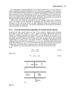
Solution: Let us consider an annular control volume with square cross-sectional area equal to
drdz centered at (r, z). Let us label the sides of the control volume R, L, T, B the centers of
which are located at (r, z + dz/2), (r, z − dz/2), (r + dr/2, z), (r − dr/2, z), respectively. In this
analysis the horizontal coordinate is z and the vertical (or radial) coordinate is r. The flow
through each of the surfaces is
m
˙R =ρ w+

∂w dz
∂z 2

2πr dr

∂w dz
2πr dr
∂z 2
∂u dr

dr
m
˙ T =ρ u+
2π r +
dz
∂r 2
2
∂u dr
dr
m
˙ B =ρ u−
2π r −
dz
∂r 2
2
The conservation of mass principle means that the net flow of mass out of the control volume
is zero, i.e.,
m
˙ R−m
˙ L+m
˙ T −m
˙B=0
m
˙L=ρ w−

This holds for both steady and unsteady conditions because ρ is assumed to be constant. An
incompressible flow is volume preserving and, hence, this result is independent of whether
or not the flow is steady. This is not the case for Euler’s equation of motion; see Exercise
2.4. Substituting the expressions for the mass flow across each part of the control surface and
rearranging terms, we get the equation given above.

(b) Show that the Stokes’s stream function ψ defined by the following expressions for the
velocity components
1 ∂ψ
1 ∂ψ
u=
, w=−
r ∂z
r ∂r
By direct substitution of these expressions into the continuity equation, we see that the continuity equation is automatically satisfied. Note that the function ψ is assumed to be a function
for which the order of differentiation is immaterial.
Problem 2.2: In this problem we want to transform the continuity equation given in (x, y)
to polar coordinates (r, φ). The two coordinate systems are related by the following formulas:
x = r cos φ. y = r sin φ. Let the components of the velocity in (x, y) be given by u = (ux , uy )
and the components in (r, φ) by u = (u, v). Note that
ux = u cos φ − v sin φ,
We want to transform

uy = u sin φ + v cos φ

∂ux ∂uy
+
=0
∂x
∂y


to the following form:
∂u u 1 ∂v
+ +
=0

∂r
r
r ∂φ
What we need to recall is that the derivative of any property f transforms as follows:
∂f
∂f ∂r
∂f ∂φ
=
+
∂x
∂r ∂x ∂φ ∂x
∂f
∂f ∂r ∂f ∂φ
=
+
∂y
∂r ∂y ∂φ ∂y
From x = r cos φ and y = r sin φ we get
∂x
∂r
∂φ
=
cos φ − r sin φ
∂x
∂x
∂x
∂y
∂r
∂φ
=

sin φ + r cos φ
∂y
∂y
∂y
Since r2 = x2 + y 2
2r

∂r
= 2x,
∂x

2r

∂r
= 2y
∂y

Hence,
∂r
= cos φ,
∂x

∂r
= sin φ
∂y

Thus,
1 − cos2 φ
sin φ
∂φ

=−
=−
,
∂x
r sin φ
r

∂φ
1 − sin2 φ
cos φ
=
=
∂y
r cos φ
r

Applying these formulas, we get
∂ux
∂ (u cos φ − v sin φ) sin φ ∂ (u cos φ − v sin φ)
= cos φ
−
∂x
∂r
r
∂φ
∂uy
∂ (u sin φ + v cos φ) cos φ ∂ (u sin φ + v cos φ)
= sin φ
+
∂y

∂r
r
∂φ
Adding these equations and equating them to zero, we get the result sought.
Extension 1 of Problem 2.2 (see also Problem 2.7): The condition for irrotationality for
two-dimensional planar flows in an (x, y) Cartesian coordinate system is:
∂v
∂u
−
= 0.
∂x ∂y
Transform this relationships to cylindrical polar coordinates, (r, θ), by checking and applying
the following transformation relationships:
x = r cos θ,

y = r sin θ.

Note that:
u = ur cos θ − uθ sin θ,
and
v = ur sin θ + uθ cos θ.
Also note that

∂f
∂f
sin θ ∂f
= cos θ
−
.
∂x

∂r
r ∂θ
2


∂f
∂f
cos θ ∂f
= sin θ
+
.
∂y
∂r
r ∂θ
The solution is

1 ∂ur
∂uθ
uθ
−
+
r ∂θ
∂r
r
Extension 2 of Problem 2.2 (see also Section 3.2.2): The second-derivative transformation
equations are as follows:
2
sin2 θ ∂f
2 cos θ sin θ
∂2f

sin2 θ ∂ 2 f
2 ∂ f
=
cos
θ
+
+
+
∂x2
∂r2
r ∂r
r2 ∂θ2
r

1 ∂f
∂2f
−
r ∂θ
∂r∂θ

.

2
cos2 θ ∂f
cos2 θ ∂ 2 f
2 sin θ cos θ
∂2f
2 ∂ f
=
sin

θ
+
+
−
∂y 2
∂r2
r ∂r
r2 ∂θ2
r

∂2f
1 ∂f
−
r ∂θ
∂r∂θ

.

The second derivative relationships are useful for transforming
∂2φ ∂2φ
+ 2 =0
∂x2
∂y
to polar coordinates. By substituting f = φ in the second-derivative relations and adding the
two resulting equations, we get
∂ 2 φ 1 ∂φ
1 ∂2φ
+
+
=0

∂r2
r ∂r
r2 ∂θ2

Problem 2.3: Sections 2.4 and 2.6 on continuity and momentum equations, respectively, are
useful. The procedure based on control-volume analysis is applied to derive the continuity and
momentum equations. The same procedure can be applied to derive the convection-diffusion
equation for C in this problem.
Assume that none of the contaminant is created within the flow field. Assume that the
transport of the contaminant matter is by convection and diffusion. In part (a) we assume that
the velocity field is unchanged and, hence, the contaminant must be sufficiently dilute. If this
is not the case, then the density of the fluid containing the contaminant could be changed in
such a way as to alter the motion of the fluid in an analogous way as when temperature changes
in a fluid are sufficient to cause hot air or hot water to naturally rise above cold air or cold
water. This is the key concept that leads to pointing out in the problem statement that the
contaminant is dilute.
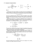
The rate of increase in C in an infinitesimal control volume like the one drawn in Fig. 2.20
in the text is
∂C
δx δy × 1
∂t
The net convective transport of C across the boundary of the control volume in Fig. 2.20 is,
substituting C for ρu, the horizontal component of the momentum, in Eq. (2.62a) and assuming
u = (u, v) is divergence free, we get
u

∂C
∂C
+v
∂x

∂y

δx δy × 1

The diffusion of C across the surface of the control volume is (by analogy with the development
of surface forces that led to Eq. (2.65a))
∂
∂
∂C
∂C
i+
j · −D
i+
j
∂x
∂y
∂x
∂y
3

δx δy × 1


Summing the three contributions leads to the result given in part (a). The equation is
∂C
∂C
∂C
+u
+v
=D

∂t
∂x
∂y

∂2C
∂2C
+
∂x2
∂y 2

Part (b) asks about the necessity of assuming a dilute suspension of contaminant. First of
all we assumed the flow field was unchanged. This is the key for the necessity of the assumption
that the contaminant is dilute. In addition, the diffusion coefficient may be a function of the
thermodynamic state. A first cut at dealing with this is to keep the derivatives of D in the
formula. A second step would be to take into account the changes in density of the fluid particle
to determine whether or no the changes in density are sufficient to induce natural convection.
More extensive treatments of mass transport can be found in the literature; a good source is
the book by Bird, Stewart and Lightfoot [4]. To take into account contaminant generation it
is handled like a body force term in the momentum equation. Hence, the equation in (a) is
altered as follows:
∂C
∂C
∂C
∂2C
∂2C
+u
+v
=D
+
+m

˙c
∂t
∂x
∂y
∂x2
∂y 2

Problem 2.4: In this problem we are interested in the components of the momentum equation
for an inviscid pressure-driven flow subjected to a conservative body force. Le us assume that
the control volume in this problem is the same as given in the solution of Problem 2.1. Also in
the solution of Problem 2.1 the mass rate of flow through each face of the control surface that
completely surrounds the control volume is given. Let us assume that there are two components
of an external body force applied to the element of fluid and they are the compnenets of the
vector g = (gr , gz ). Let us also assume that the only surface force acting on the surface of the
control volume is pressure. Thus, we have neglected viscous normal and shear stresses (i.e., we
assume the flow is inviscid). There are two components of the momentum equation that are
not zero because we assumed axisymmetric flow with zero swirl; as we have done in Problem
2.1. The radial and axial components of the momentum principle, respectively, are:
ρ

∂u
2πrdrdz + m
˙ R uR − m
˙ L uL + m
˙ T uT − m
˙ B uB = pL AL − pR AR + ρgr 2πrdrdz
∂t

∂w
2πrdrdz + m

˙ R wR − m
˙ L wL + m
˙ T wT − m
˙ B wB = pB AB − pT AT + ρgφ 2πrdrdz
∂t
The velocity components in these formulas are
ρ

uR = u +

∂u dz
,
∂z 2

uL = u −

∂u dz
∂z 2

∂u dr
∂u dr
, uB = u −
∂r 2
∂r 2
∂w dz
∂w dz
wR = w +
, wL = w −
∂z 2
∂z 2

∂w dr
∂w dr
wT = w +
, wB = w −
∂r 2
∂r 2
Substituting for the mass rate of flow and for the velocity components associated with each
surface of the control volume into the momentum equations above, after rearranging terms and
applying the continuity equation given in the problem statement of Problem 2.1, we get
uT = u +

ρ

∂u
∂u
∂u
+u
+w
∂t
∂r
∂z
4

=−

∂p
+ ρgr
∂r

ρ

∂w
∂w
∂w
+u
+w
∂t
∂r
∂z

=−

∂p
+ ρgz
∂z

which are the equations of motion sought. These are the components of Euler’s equation for
axisymmetric flow.
Problem 2.5: Section 2.7 gives the solution procedure. The first set is to interpret u as the
radial component of the velocity, and, hence, x as the radial coordinate, and interpret v as the
z component of the velocity (w) and, hence, y as the axial coordinate. The main additions that
need to be included are that area through the control surface perpendicular to the r direction
increases with r and is equal to 2πrdφ, where φ is the coordinate in the angular direction.
Axisymmetry implies that there are no changes in properties of the flow in the φ direction.
Also assumed is that there is no angular velocity component. This does not mean that there
is no rate of strain in the φ direction. In fact, for a fix δr and δz for r1 < r2 the control
volume is larger for r2 as compared with the control volume around r1 . Thus, transporting
the flow radially leads to ˙φφ = u/r. Otherwise, the derivation of the rates of strain follow the
development given in Section 2.7.

In Part (b) of this problem is to transform the (x, y, z) form of the Navier-Stokes equations
to cylindrical polar coordinates (r, φ, z) such that the changes in any property in φ are zero.
Also, assume the velocity vector is u = (u, 0, w) in the polar coordinates. Since differentiation
of the unit vector k, which is in the z direction, is zero, the formula for the ∇ · ∇f = ∇2 f term
given in the solution of Problem 2.2 can be applied directly to get ∇2 w, the last term in the
last equation given in the problem statement. If you take the second derivative of the first two
terms in the first equation in the problem statement of Problem 2.2, you get the correct form
for the third, fourth and fifth terms on the right hand side of the next to last equation in the
problem statement for this problem.
Problem 2.6: Euler’s equations for two-dimensional flows can be transformed from (x, y) to
(r, φ) by applying the formulas given in the solution for Problem 2.2. Of course, the body force
components must be converted from (gx , gy ) to (gr , gφ ) by similar formulas for ur and uφ given
in the solution of Problem 2.2.
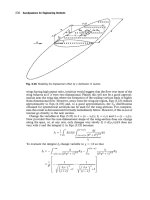
Problem 2.7: Care is required to draw the fluid particle and how it moves (as suggested
in the hint). The vorticity can be found as given in one of the extensions to the solution of
Problem 2.2. To examine the other rates of strain it may be convenient for the student to
start with the particle in Fig. 2.13. An alternative approach is to apply the transformation
equations in the solution of Problem 2.2 to the rates of strain in (x, y). The best treatment
of the transformation relations as they apply to vectors and tensors is given in an appendix in
Bird, Stewart and Lightfoot [4].
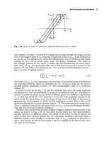
Problem 2.8: In this problem the shear stress is tangent to circles of radius r. The shear stress
is equal to τ = µRω/h. The area on which it acts is 2πr dr × L. Thus, the torque associated
with this stress (force per unit area) is dT = tan 2πr2 dr × L. This needs to be integrated from
r = 0 to r = R to obtain the formula given. The power is equal to 2πnT = T ω. This is also
what is given.
Problem 2.9: The key to this solution is to start, as indicated in the problem statement, with
the formulas for the two compnenets of the Navier-Stokes equations in cylindrical coordinates
given in Problem 2.5. You need to replace the formula for v to v = −az/ζ 2 . This is to take
into account the fact that areas perpendicular to r are equal to 2πr. Otherwise, the method is
exactly what is presented in Section 2.10.3.

5


Solutions manual & MATLAB files
for
Aerodynamics for engineering students, sixth edition
ISBN: 978-0-08-096632-8 (pbk.)
TL570.H64 2012
629.132’5dc23
March 2012
E. L. Houghton, P. W. Carpenter, Steven H. Collicott
and
Daniel T. Valentine

Chapter 2 Solutions to many if the end-of-chapter problems.


D.T. Valentine

AMSTERDAM • BOSTON • HEIDELBERG • LONDON
NEW YORK • OXFORD • PARIS • SAN DIEGO
SAN FRANCISCO • SINGAPORE • SYDNEY • TOKYO
Butterworth-Heinemann is an imprint of Elsevier

To protect the rights of the author(s) and publisher we inform you that this PDF is an uncorrected proof for internal business use only by the author(s), editor(s),
reviewer(s), Elsevier and typesetter diacriTech. It is not allowed to publish this proof online or in print. This proof copy is the copyright property of the publisher
and is confidential until formal publication.

SOLUTIONS MANUAL

Houghton — FM-9780080966328 — 2012/1/17 — 22:00 — Page iii — #3

Aerodynamics for
Engineering Students
Sixth Edition

E.L. Houghton
P.W. Carpenter
S.H. Collicott
D.T. Valentine

AMSTERDAM • BOSTON • HEIDELBERG • LONDON
NEW YORK • OXFORD • PARIS • SAN DIEGO
SAN FRANCISCO • SINGAPORE • SYDNEY • TOKYO
Butterworth-Heinemann is an imprint of Elsevier


1

Solutions to Chapter 2 problems

This section provides solutions for typical homework problems at the end of Chapter 2.
Problem 2.1: In this problem we are interested in the continuity equation for axisymmetric
flow in terms of the cylindrical coordinate system (r, φ, z), where all flow variables are independent of angular coordinate, φ. Let the velocity components (u, v, w) = (u, 0, w) in the (r, φ, z)
coordinate directions. (a) Show that the continuity equation is given by
∂u u ∂w
+ +
=0
∂r
r

∂z
Solution: Let us consider an annular control volume with square cross-sectional area equal to
drdz centered at (r, z). Let us label the sides of the control volume R, L, T, B the centers of
which are located at (r, z + dz/2), (r, z − dz/2), (r + dr/2, z), (r − dr/2, z), respectively. In this
analysis the horizontal coordinate is z and the vertical (or radial) coordinate is r. The flow
through each of the surfaces is
m
˙R =ρ w+

∂w dz
∂z 2

2πr dr

m
˙L=ρ w−

∂w dz
∂z 2

2πr dr

m
˙ T =ρ u+

∂u dr
∂r 2

2π r +

dr
2

dz

m
˙ B =ρ u−

∂u dr
∂r 2

2π r −

dr
2

dz

The conservation of mass principle means that the net flow of mass out of the control volume
is zero, i.e.,
m
˙ R−m
˙ L+m
˙ T −m
˙B=0
This holds for both steady and unsteady conditions because ρ is assumed to be constant. An
incompressible flow is volume preserving and, hence, this result is independent of whether
or not the flow is steady. This is not the case for Euler’s equation of motion; see Exercise
2.4. Substituting the expressions for the mass flow across each part of the control surface and
rearranging terms, we get the equation given above.

(b) Show that the Stokes’s stream function ψ defined by the following expressions for the
velocity components
1 ∂ψ
1 ∂ψ
u=
, w=−
r ∂z
r ∂r
By direct substitution of these expressions into the continuity equation, we see that the continuity equation is automatically satisfied. Note that the function ψ is assumed to be a function
for which the order of differentiation is immaterial.
Problem 2.2: In this problem we want to transform the continuity equation given in (x, y)
to polar coordinates (r, φ). The two coordinate systems are related by the following formulas:
x = r cos φ. y = r sin φ. Let the components of the velocity in (x, y) be given by u = (ux , uy )
and the components in (r, φ) by u = (u, v). Note that
ux = u cos φ − v sin φ,

uy = u sin φ + v cos φ


We want to transform

∂ux ∂uy
+
=0
∂x
∂y

to the following form:
∂u u 1 ∂v
+ +

=0
∂r
r
r ∂φ
What we need to recall is that the derivative of any property f transfprms as follows:
∂f
∂f ∂r
∂f ∂φ
=
+
∂x
∂r ∂x ∂φ ∂x
∂f
∂f ∂r ∂f ∂φ
=
+
∂y
∂r ∂y ∂φ ∂y
From x = r cos φ and y = r sin φ we get
∂x
∂r
∂φ
=
cos φ − r sin φ
∂x
∂x
∂x
∂y
∂r
∂φ

=
sin φ + r cos φ
∂y
∂y
∂y
Since r2 = x2 + y 2
2r

∂r
= 2x,
∂x

2r

∂r
= 2y
∂y

Hence,
∂r
= cos φ,
∂x

∂r
= sin φ
∂y

Thus,
∂φ
1 − cos2 φ

sin φ
=−
=−
,
∂x
r sin φ
r

∂φ
1 − sin2 φ
cos φ
=
=
∂y
r cos φ
r

Applying these formulas, we get
∂ux
∂ (u cos φ − v sin φ) sin φ ∂ (u cos φ − v sin φ)
= cos φ
−
∂x
∂r
r
∂φ
∂ (u sin φ + v cos φ) cos φ ∂ (u sin φ + v cos φ)
∂uy
= sin φ
+

∂y
∂r
r
∂φ
Adding these equations and equating them to zero, we get the result sought.
Problem 2.4: In this problem we are interested in the components of the momentum equation
for an inviscid pressure-driven flow subjected to a conservative body force. Le us assume that
the control volume in this problem is the same as given in the solution of Problem 2.1. Also in
the solution of Problem 2.1 the mass rate of flow through each face of the control surface that
completely surrounds the control volume is given. Let us assume that there are two components
of an external body force applied to the element of fluid and they are the compnenets of the
vector g = (gr , gz ). Let us also assume that the only surface force acting on the surface of the
control volume is pressure. Thus, we have neglected viscous normal and shear stresses (i.e., we
assume the flow is inviscid). There are two components of the momentum equation that are
not zero because we assumed axisymmetric flow with zero swirl; as we have done in Problem
2.1. The radial and axial components of the momentum principle, respectively, are:
ρ

∂u
2πrdrdz + m
˙ R uR − m
˙ L uL + m
˙ T uT − m
˙ B uB = pL AL − pR AR + ρgr 2πrdrdz
∂t
2


∂w
2πrdrdz + m

˙ R wR − m
˙ L wL + m
˙ T wT − m
˙ B wB = pB AB − pT AT + ρgφ 2πrdrdz
∂t
The velocity components in these formulas are
ρ

uR = u +

∂u dz
,
∂z 2

uL = u −

∂u dz
∂z 2

∂u dr
∂u dr
, uB = u −
∂r 2
∂r 2
∂w dz
∂w dz
wR = w +
, wL = w −
∂z 2
∂z 2

∂w dr
∂w dr
wT = w +
, wB = w −
∂r 2
∂r 2
Substituting for the mass rate of flow and for the velocity components associated with each
surface of the control volume into the momentum equations above, after rearranging terms and
applying the continuity equation given in the problem statement of Problem 2.1, we get
uT = u +

ρ

∂u
∂u
∂u
+u
+w
∂t
∂r
∂z

=−

ρ

∂w
∂w
∂w
+u

+w
∂t
∂r
∂z

=−

∂p
+ ρgr
∂r
∂p
+ ρgz
∂z

which are the equations of motion sought. These are the components of Euler’s equation for
axisymmetric flow.

3