Test bank and solution of nature of cost (1)

Chapter_2_9e_Solutions.pdf
ZimmermanCh02.pdf


CHAPTER 2
THE NATURE OF COSTS
P 2-1:

Solution to Darien Industries (10 minutes)
[Relevant costs and benefits]
Current cafeteria income
Sales
Variable costs (40% × 12,000)
Fixed costs
Operating income
Vending machine income
Sales (12,000 × 1.4)
Darien's share of sales
(.16 × $16,800)
Increase in operating income

P 2-2:

$12,000
(4,800)
(4,700)
$2,500
$16,800
2,688
$ 188

Negative Opportunity Costs (10 minutes)
[Opportunity cost]

Yes, when the most valuable alternative to a decision is a net cash outflow that
would have occurred is now eliminated. The opportunity cost of that decision is negative
(an opportunity benefit). For example, suppose you own a house with an in-ground
swimming pool you no longer use or want. To dig up the pool and fill in the hole costs
$3,000. You sell the house instead and the new owner wants the pool. By selling the
house, you avoid removing the pool and you save $3,000. The decision to sell the house
includes an opportunity benefit (a negative opportunity cost) of $3,000.
P 2-3:

Solution to NPR (10 minutes)
[Opportunity cost of radio listeners]

The quoted passage ignores the opportunity cost of listeners’ having to forego
normal programming for on-air pledges. While such fundraising campaigns may have a
low out-of-pocket cost to NPR, if they were to consider the listeners’ opportunity cost,
such campaigns may be quite costly.

Chapter 2
Instructor’s Manual, Accounting for Decision Making and Control

© McGraw-Hill Education 2017
2-1


P 2-4:

Solution to Silky Smooth Lotions (15 minutes)

[Break even with multiple products]

Given that current production and sales are: 2,000, 4,000, and 1,000 cases of 4, 8,
and 12 ounce bottles, construct of lotion bundle to consist of 2 cases of 4 ounce bottles, 4
cases of 8 ounce bottles, and 1 case of 12 ounce bottles. The following table calculates
the break-even number of lotion bundles to break even and hence the number of cases of
each of the three products required to break even.

Per Case
Price
Variable cost
Contribution margin
Current production

4 ounce
$36.00
$13.00
$23.00
2000

8 ounce
$66.00
$24.50
$41.50
4000

12 ounce
$72.00
$27.00
$45.00

1000

2

4

1

$46.00

$166.00

$45.00

Cases per bundle
Contribution margin per bundle
Fixed costs

Bundle

$257.00
$771,000

Number of bundles to break even
Number of cases to break even
P 2-5:

3000
6000

12000

3000

Solution to J. P. Max Department Stores (15 minutes)
[Opportunity cost of retail space]

Profits after fixed cost allocations
Allocated fixed costs
Profits before fixed cost allocations
Lease Payments
Forgone Profits

Home Appliances Televisions
$64,000
$82,000
7,000
8,400
71,000
90,400
72,000
86,400
– $1,000
$ 4,000

We would rent out the Home Appliance department, as lease rental receipts are
more than the profits in the Home Appliance Department. On the other hand, profits
generated by the Television Department are more than the lease rentals if leased out, so
we continue running the TV Department. However, neither is being charged inventory
holding costs, which could easily change the decision.

Also, one should examine externalities. What kind of merchandise is being sold
in the leased store and will this increase or decrease overall traffic and hence sales in the
other departments?
Chapter 2
2-2

© McGraw-Hill Education 2017
Instructor’s Manual, Accounting for Decision Making and Control


P 2-6:
a.

Solution to Vintage Cellars (15 minutes)
[Average versus marginal cost]
The following tabulates total, marginal and average cost.
Quantity
1
2
3
4
5
6
7
8
9
10

Average
Cost

$12,000
10,000
8,600
7,700
7,100
7,100
7,350
7,850
8,600
9,600

Total Marginal
Cost
Cost
$12,000
20,000
$8,000
25,800
5,800
30,800
5,000
35,500
4,700
42,600
7,100
51,450
8,850
62,800
11,350
77,400

14,600
96,000
18,600

b.

Marginal cost intersects average cost at minimum average
(MC=AC=$7,100). Or, at between 5 and 6 units AC = MC = $7,100.

c.

At four units, the opportunity cost of producing and selling one more unit is
$4,700. At four units, total cost is $30,800. At five units, total cost rises to
$35,500. The incremental cost (i.e., the opportunity cost) of producing the fifth
unit is $4,700.

d.

Vintage Cellars maximizes profits ($) by producing and selling seven units.
Quantity
1
2
3
4
5
6
7
8
9
10

P 2-7:

Average
Cost
$12,000
10,000
8,600
7,700
7,100
7,100
7,350
7,850
8,600
9,600

Total
Cost
$12,000
20,000
25,800
30,800
35,500
42,600
51,450
62,800
77,400
96,000

Total

Revenue
$9,000
18,000
27,000
36,000
45,000
54,000
63,000
72,000
81,000
90,000

cost

Profit
-$3,000
-2,000
1,200
5,200
9,500
11,400
11,550
9,200
3,600
-6,000

Solution to ETB (15 minutes)
[Minimizing average cost does not maximize profits]

a.

The following table calculates that the average cost of the iPad bamboo case is
minimized by producing 4,500 cases per month.
Chapter 2
Instructor’s Manual, Accounting for Decision Making and Control

© McGraw-Hill Education 2017
2-3


Production (units)
Total cost
Average cost
b.

Monthly Production and Sales
3,000
3,500
4,500
5,000
$162,100 $163,000 $167,500 $195,000
$54.03

$46.57

$37.22

$39.00

The following table calculates net income of the four production (sales) levels.

Production (units)

Monthly Production and Sales
3,000
3,500
4,500
5,000

Revenue
Total cost
Net income

$195,000 $227,500 $292,500 $325,000
162,100 163,000 167,500 195,000
$32,900 $64,500 $125,000 $130,000

Based on the above analysis, the profit maximizing production (sales) level is to
manufacture and sell 5,000 iPad cases a month. Selecting the output level that minimizes
average cost (4,500 cases) does not maximize profits.
P 2-8:
a.

Solution to Taylor Chemicals (15 minutes)
[Relation between average, marginal, and total cost]
Marginal cost is the cost of the next unit. So, producing two cases costs an
additional $400, whereas to go from producing two cases to producing three cases
costs an additional $325, and so forth. So, to compute the total cost of producing
say five cases you sum the marginal costs of 1, 2, …, 5 cases and add the fixed
costs ($500 + $400 + $325 + $275 + $325 + $1000 = $2825). The following table
computes average and total cost given fixed cost and marginal cost.

Chapter 2
2-4

© McGraw-Hill Education 2017
Instructor’s Manual, Accounting for Decision Making and Control


Quantity

Marginal
Cost

Fixed
Cost

Total
Cost

Average
Cost

1

$500

$1000

$1500

$1500.00

2

400

1000

1900

950.00

3

325

1000

2225

741.67

4

275

1000

2500

625.00

5

325

1000

2825

565.00

6

400

1000

3225

537.50

7

500

1000

3725

532.14

8

625

1000

4350

543.75

9

775

1000

5125

569.44

10

950

1000

6075

607.50

b.

Average cost is minimized when seven cases are produced. At seven cases,
average cost is $532.14.

c.

Marginal cost always intersects average cost at minimum average cost. If
marginal cost is above average cost, average cost is increasing. Likewise, when
marginal cost is below average cost, average cost is falling. When marginal cost
equals average cost, average cost is neither rising nor falling. This only occurs
when average cost is at its lowest level (or at its maximum).

P 2-9:

Solution to Emrich Processing (15 minutes)
[Negative opportunity costs]

Opportunity costs are usually positive. In this case, opportunity costs are negative
(opportunity benefits) because the firm can avoid disposal costs if they accept the rush
job.
The original $1,000 price paid for GX-100 is a sunk cost. The opportunity cost of
GX-100 is -$400. That is, Emrich will increase its cash flows by $400 by accepting the
rush order because it will avoid having to dispose of the remaining GX-100 by paying
Environ the $400 disposal fee.
How to price the special order is another question. Just because the $400 disposal
fee was built into the previous job does not mean it is irrelevant in pricing this job.
Clearly, one factor to consider in pricing this job is the reservation price of the customer

proposing the rush order. The $400 disposal fee enters the pricing decision in the
following way: Emrich should be prepared to pay up to $399 less any out-of-pocket
costs to get this contract.

Chapter 2
Instructor’s Manual, Accounting for Decision Making and Control

© McGraw-Hill Education 2017
2-5


P 2-10:

Solution to Verdi Opera or Madonna? (15 minutes)
[Opportunity cost of attending a Madonna concert]

If you attend the Verdi opera, you forego the $200 in benefits (i.e., your willingness
to pay) you would have received from going to see Madonna. You also save the $160
(the costs) you would have paid to see Madonna. Since an avoided benefit is a cost and
an avoided cost is a benefit, the opportunity cost of attending the opera (the value you
forego by not attending the Madonna concert) is $40 – i.e., the net benefit foregone. Your
willingness to pay $30 for the Verdi opera is unrelated to the costs and benefits of
foregoing the Madonna concert.
P 2-11:

Solution to Dod Electronics (15 minutes)
[Estimating marginal cost from average cost]

Dod should accept Xtron’s offer. The marginal cost to produce the 10,000 chips is
unknown. But since management is convinced that average cost is falling, this means

that marginal cost is less than average cost. The only way that average cost of $35
can fall is if marginal cost is less than $35. Since Xtron is willing to pay $38 per
chip, Dod should make at least $30,000 on this special order (10,000 x $3). This
assumes (i) that average cost continues to fall for the next 10,000 units (i.e., it
assumes that at, say 61,000 units, average cost does not start to increase), and (ii)
there are no other costs of taking this special order.
b. Dod can’t make a decision based on the information. Since average cost is
increasing, we know that marginal cost is greater than $35 per unit. But we don’t
know how much larger. If marginal cost at the 60,001th unit is $35.01, average cost
is increasing and if marginal cost of the 70,000th unit is less than $38, then DOD
should accept the special order. But if marginal cost at the 60,001th unit is $38.01,
the special order should be rejected.
a.

P 2-12:

Solution to Napoli Pizzeria (15 minutes)
[Break-even analysis]

a. The break-even number of servings per month is:
($300 – $75) ÷ ($3 – $1)
= ($225) ÷ ($2)
= 112.5 servings
b. To generate $1,000 after taxes Gino needs to sell 881.73 servings of
espresso/cappuccino.
Profits after tax = [Revenues – Expenses] x (1– 0.35)
$1,000 = [$3N + $75 – $1N – $300] x (1– 0.35)
$1,000 = [$2N – $225] x .65
$1,000 ÷ .65 = $2N – $225
Chapter 2

2-6

© McGraw-Hill Education 2017
Instructor’s Manual, Accounting for Decision Making and Control


$1,538.46 = $2N – $225
$2N = $1,763.46
N = 881.73
P 2-13:

a.

Solution to JLT Systems (20 minutes)
[Cost-volume-profit analysis]

Since we know that average cost is $2,700 at 200 unit sales, then Total Cost (TC)
divided by 200 is $2,700. Also, since JLT has a linear cost curve, we can write,
TC=FC+VxQ where FC is fixed cost, V is variable cost per unit, and Q is quantity
sold and installed. Given FC = $400,000, then:
TC/Q = (FC+VxQ)/Q = AC
($400,000 + 200 V) / 200 = $2,700
$400,000 + 200 V = $540,000
200 V = $140,000
V = $700

b.

Given the total cost curve from part a, a tax rate of 40%, and a $2,000 selling
price, and an after-tax profit target of $18,000, we can write:

($2000 Q - $400,000 - $700 Q) x (1- 40%) = $18,000
1300 Q -400,000 = 18,000 / .60 = 30,000
1300 Q = 430,000
Q = 330.8
In other words, to make an after-tax profit of $18,000, JLT must have 330.8 sales
and installs per month.

c.

The simplest (and fastest way) to solve for the profit maximizing quantity given
the demand curve is to write the profit equation, take the first derivative, set it to
zero, and solve for Q.
Total Profit = (2600 - 2Q) Q -400,000 -700 Q
First derivative: 2600 - 4Q -700 = 0
4Q = 1900
Q = 475
The same solution is obtained if you set marginal revenue (where MR is 2600 4Q) equal to marginal cost (700), and again solve for Q, or
2600 - 4Q = 700
Q = 475
The more laborious solution technique is to use a spreadsheet and identify the
profit maximizing price quantity combination.

Chapter 2
Instructor’s Manual, Accounting for Decision Making and Control

© McGraw-Hill Education 2017
2-7


Quantity

250
275
300
325
350
375
400
425
450
475
500
525
550

Price
$2,100
2,050
2,000
1,950
1,900
1,850
1,800
1,750
1,700
1,650
1,600
1,550
1,500

Revenue

$525,000
563,750
600,000
633,750
665,000
693,750
720,000
743,750
765,000
783,750
800,000
813,750
825,000

Total Cost
$575,000
592,500
610,000
627,500
645,000
662,500
680,000
697,500
715,000
732,500
750,000
767,500
785,000

Profit

($50,000)
(28,750)
(10,000)
6,250
20,000
31,250
40,000
46,250
50,000
51,250
50,000
46,250
40,000

As before, we again observe that 475 sales and installs maximize profits.
P 2-14:

Solution to Volume and Profits (15 minutes)
[Cost-volume-profit]

a.

False.

b.

Write the equation for firm profits:
Profits = P × Q - (FC - VC × Q) = Q(P - VC) - FC
= Q(P - VC) - (FC ÷ Q)Q
Notice that average fixed costs per unit (FC÷Q) falls as Q increases, but with

more volume, you have more fixed cost per unit such that (FC÷Q) × Q = FC.
That is, the decline in average fixed cost per unit is exactly offset by having more
units.
Profits will increase with volume even if the firm has no fixed costs, as
long as price is greater than variable costs. Suppose price is $3 and variable cost
is $1. If there are no fixed costs, profits increase $2 for every unit produced.
Now suppose fixed cost is $50. Volume increases from 100 units to 101 units.
Profits increase from $150 ($2 ×100 - $50) to $152 ($2 × 101 - $50). The change
in profits ($2) is the contribution margin. It is true that average unit cost declines
from $1.50 ([100 × $1 + $50]÷100) to $1.495 ([101 × $1 + $50]÷101). However,
this has nothing to do with the increase in profits. The increase in profits is due
solely to the fact that the contribution margin is positive.

Chapter 2
2-8

© McGraw-Hill Education 2017
Instructor’s Manual, Accounting for Decision Making and Control


Alternatively, suppose price is $3, variable cost is $3, and fixed cost is
$50. Contribution margin in this case is zero. Doubling output from 100 to 200
causes average cost to fall from $3.50 ([100 × $3 + $50]÷100) to $3.25 ([200 × $3
+ $50]÷200), but profits are still zero.
P 2-15:
a.

Solution to American Cinema (20 minutes)
[Break-even analysis for an operating decision]

Both movies are expected to have the same ticket sales in weeks one and two, and
lower sales in weeks three and four.
Let Q1 be the number of tickets sold in the first two weeks, and Q2 be the number
of tickets sold in weeks three and four. Then, profits in the first two weeks, 1,
and in weeks three and four, 2, are:
1 = .1(6.5Q1) – $2,000
2 = .2(6.5Q2) – $2,000
―I Do‖ should replace ―Paris‖ if
1 > 2, or
.65Q1 – 2,000 > 1.3Q2 – 2,000, or
Q1 > 2Q2.
In other words, they should keep ―Paris‖ for four weeks unless they expect ticket
sales in weeks one and two of ―I Do‖ to be twice the expected ticket sales in
weeks three and four of ―Paris.‖

b.

Taxes of 30 percent do not affect the answer in part (a).

c.

With average concession profits of $2 per ticket sold,
1 = .65Q1 + 2Q1 – 2,000
2 = 1.30Q2 + 2Q2 – 2,000
1 > 2 if
2.65Q1 > 3.3Q2
Q1 > 1.245Q2

Chapter 2
Instructor’s Manual, Accounting for Decision Making and Control

© McGraw-Hill Education 2017
2-9


Now, ticket sales in the first two weeks need only be about 25 percent higher than
in weeks three and four to replace ―Paris‖ with ―I Do.‖
P 2-16:
a.

Solution to Home Auto Parts (20 minutes)
[Opportunity cost of retail display space]

The question involves computing the opportunity cost of the special promotions
being considered. If the car wax is substituted, what is the forgone profit from the
dropped promotion? And which special promotion is dropped? Answering this
question involves calculating the contribution of each planned promotion. The
opportunity cost of dropping a planned promotion is its forgone contribution:
(retail price less unit cost) × volume. The table below calculates the expected
contribution of each of the three planned promotions.
Planned Promotion Displays
For Next Week
End-ofAisle
Texcan Oil

Front
Door
Wiper blades

Cash

Register
Floor mats

5,000

200

70

69¢/can

$9.99

$22.99

Unit cost

62¢

$7.99

$17.49

Contribution margin

7¢

$2.00

$5.50

$350

$400

$385

Item
Projected volume (week)
Sales price

Contribution
(margin × volume)

Texcan oil is the promotion yielding the lowest contribution and therefore is the
one Armadillo must beat out. The contribution of Armadillo car wax is:
Selling price
less: Unit cost
Contribution margin
× expected volume
Contribution

Chapter 2
2-10

$2.90
$2.50
$0.40
800
$ 320

© McGraw-Hill Education 2017
Instructor’s Manual, Accounting for Decision Making and Control


Clearly, since the Armadillo car wax yields a lower contribution margin than all
three of the existing planned promotions, management should not change their
planned promotions and should reject the Armadillo offer.
b.

With 50 free units of car wax, Armadillo’s contribution is:
Contribution from 50 free units (50 × $2.90)
Contribution from remaining 750 units:
Selling price
$2.90
less: Unit cost
$2.50
Contribution margin
$0.40
× expected volume
750
Contribution

$145

300
$445

With 50 free units of car wax, it is now profitable to replace the oil display area
with the car wax. The opportunity cost of replacing the oil display is its forgone

contribution ($350), whereas the benefits provided by the car wax are $445.
Additional discussion points raised
(i)

This problem introduces the concept of the opportunity cost of retail shelf
space. With the proliferation of consumer products, supermarkets’
valuable scarce commodity is shelf space. Consumers often learn about a
product for the first time by seeing it on the grocery shelf. To induce the
store to stock an item, food companies often give the store a number of
free cases. Such a giveaway compensates the store for allocating scarce
shelf space to the item.

(ii)

This problem also illustrates that retail stores track contribution margins
and volumes very closely in deciding which items to stock and where to
display them.

(iii)

One of the simplifying assumptions made early in the problem was that
the sale of the special display items did not affect the unit sales of
competitive items in the store. Suppose that some of the Texcan oil sales
came at the expense of other oil sales in the store. Discuss how this would
alter the analysis.

P 2-17:

Solution to Stahl Inc. (25 minutes)
[Finding unknown quantities in cost-volume-profit analysis]

The formula for the break-even quantity is
Break-even
where:

Q = Fixed Costs / (P - V)
P = price per unit

Chapter 2
Instructor’s Manual, Accounting for Decision Making and Control

© McGraw-Hill Education 2017
2-11


V = variable cost per unit
Substituting the data into this equation yields
24,000 = F / (P - 12)
F = 24,000 P - 288,000

(1)

From the after tax data we can write down the following equation:
Profits after tax = (1-T) (P Q - V Q - Fixed Cost)
Where T = tax rate = 0.30
33,600 = (1 - 0.30) (30,000 P - 30,000 V - F)
33,600 = 0.70 (30,000 P - 30,000 x 12 - F)
48,000 =30,000 P - 360,000 - F
Substituting in eq. (1) from above yields:
48,000 =30,000 P - 360,000 - (24,000 P - 288,000)

408,000 =30,000 P - 24,000 P + 288,000
P = $20
Substituting P = $20 back into eq. (1) from above yields:
F = 24,000 x 20 - 288,000
F = $192,000
P 2-18:
a.

Solution to Affording a Hybrid (20 minutes)
[Break-even analysis]

The $1,500 upfront payment is irrelevant since it applies to both alternatives. To
find the break-even mileage, M, set the monthly cost of both vehicles equal:
 $3.00 
 $3.00 
$499  M 
  $399  M 

 50 
 25 

$100

= M(.12 - .06)

M = $100/.06 = 1,666.66 miles per month
Miles per year = 1,666.66 × 12 = 20,000
b.

 $4.00 

 $4.00 
$499  M 
  399  M 

 50 
 25 

$100 = M(.16 - .08)
Chapter 2
2-12

© McGraw-Hill Education 2017
Instructor’s Manual, Accounting for Decision Making and Control


M = $100/.08 = 1,250 miles per month
Miles per year = 1,250 × 12 = 15,000 miles per year
P 2-19:
a.

Solution to Easton Diagnostics (20 minutes)
[Break-even and operating leverage]

As computed in the following table, if the proposal is accepted, the break-even
point falls from 7,000 blood samples to 6,538 samples as computed in the
following table:
Current
Equipment
$750

Proposed
equipment
$750

175
125
150
$450

175
135
180
$490

$1,600,000
400,000
100,000
$2,100,000

$1,200,000
400,000
100,000
$1,700,000

Contribution margin

$300

$260

Break-even

7,000

6,538

Price
Variable costs:
Direct labor
Direct material
Royalty fee
Total variable costs
Fixed costs:
Lease
Supervision
Occupancy costs
Fixed costs

b.

The table below shows that at an annual volume of 10,300 blood samples, Easton
makes $12,000 more by staying with its existing equipment than by accepting the
competing vendor’s proposal. However, such a recommendation ignores the fact
that staying with the existing lease adds $400,000 of operating leverage to Easton
compared to the vendor’s proposal, thereby increasing the chance of financial
distress. If Easton has sufficient net cash flow that the chance of financial distress
is very remote, then there is no reason to worry about the higher operating
leverage of the existing lease and management should reject the proposal.
However, if Easton’s net cash flow has significant variation such that financial
distress is a concern, then the proposed equipment lease that lowers operating

leverage by $400,000 should be accepted if the expected costs of financial distress
fall by more than $12,000 per year.

Chapter 2
Instructor’s Manual, Accounting for Decision Making and Control

© McGraw-Hill Education 2017
2-13


Price
Total variable costs
Contribution margin
Fixed costs
Annual volume
Total profit

P2-20:

Current
Equipment
$750
450
$300

Proposed
equipment
$750
490
$260

$2,100,000

$1,700,000

10,300
$990,000

10,300
$978,000

Solution to Spa Salon (20 minutes)
[Break-even analysis with two products]

The problem states that the Spa performed 90 massages and 30 manicures last
month. From these data and the revenue numbers we can compute the price of a massage
is $90 ($8,100 / 90) and the price of a manicure is $50 ($1,500 /30). Similarly, the
variable cost of a massage is $40 ($3,600/90) and a manicure is $20 ($600/30),
respectively.
Since one out of every three massage clients also purchases a manicure, a bundle
of products consists of 3 massages and one manicure (with revenues of $320 = 3 × $90 +
$50 and variable cost of $140 = 3 × $40 + 20).
We can now compute the break-even number of bundles as
Break-even bundles = FC/(P-VC) = $7,020/($320-$140)
= 39 bundles
39 bundles consists of 39 × 3 massages
39 bundles consists of 39 × 1 manicures

= 117 massages
= 39 manicures

To check these computations, prepare an income statement using 117
massages and 39 manicures
Massage revenue (117 × $90)
Manicure revenue (39 × $50)
Total revenue
Massage variable cost (117 × $40)
Manicure variable cost (39 × $20)
Fixed cost
Total costs
Profit

Chapter 2
2-14

$10,530
1,950
$12,480
4680
780
7,020
$12,480
$0

© McGraw-Hill Education 2017
Instructor’s Manual, Accounting for Decision Making and Control


P 2-21:

Solution to Manufacturing Cost Classification (20 minutes)
[Period versus product costs]

Advertising expenses for DVD
Depreciation on PCs in marketing dept.
Fire insurance on corporate headquarters
Fire insurance on plant
Leather carrying case for the DVD
Motor drive (externally sourced)
Overtime premium paid assembly workers
Plant building maintenance department
Plant security guards
Plastic case for the DVD
Property taxes paid on corporate office
Salaries of public relations staff
Salary of corporate controller
Wages of engineers in quality control dept.
Wages paid assembly line employees
Wages paid employees in finished goods
warehouse

P 2-22:
a.

Period
Cost
x
x
x

Product
Cost

Direct
Labor

x
x
x
x
x
x
x

Direct
Material

Overhead

x
x
x
x
x
x
x

x
x
x

x
x

x
x

x

Solution to Australian Shipping (20 minutes)
[Negative transportation costs]

Recommendation: The ship captain should be indifferent (at least financially)
between using stone or wrought iron as ballast. The total cost (£550) is the same.
Stone as ballast
Cost of purchasing and loading stone
Cost of unloading and disposing of stone
Ton required
Total cost
Wrought iron as ballast
Number of bars required:
10 tons of ballast × 2,000 pounds/ton
Weight of bar
Loss per bar (£1.20 – £0.90)
× number of bars
Cost of loading bars (£15 ×10)
Cost of unloading bars (£10 ×10)

Chapter 2
Instructor’s Manual, Accounting for Decision Making and Control

£40
15
£55
× 10
£550

20,000 pounds
÷ 20 pounds/bar
1,000 bars
£0.30
1,000
£300
150
100
© McGraw-Hill Education 2017
2-15


Total cost
b.

£550

The price is lower in Sydney because the supply of wrought iron relative to
demand is greater in Sydney because of wrought iron’s use as ballast. In fact, in
equilibrium, ships will continue to import wrought iron as ballast as long as the
relative price of wrought iron in London and Sydney make it cheaper (net of
loading and unloading costs) than stone.

P 2-23:

Solution to iGen3 (20 minutes)
[Cost-volume-profit and break-even on a lease contract]

a and b. Break-even number of impressions under Options A and B:
Option A
$10,000
5,000
$15,000

Monthly fixed lease cost
Labor/month
Total fixed cost/month
Variable lease cost/impression
Ink/impression
Total variable cost

$0.01
0.02
$0.03

$0.03
0.02
$0.05

Price/impression

$0.08

$0.08

$0.05
300,000

$0.03
166,667

Contribution margin/impression
Break-even number of impressions
c.

Option B
$0
5,000
$5,000

The choice of Option A or B depends on the expected print volume ColorGrafix
forecasts. Choosing among different cost structures should not be based on
break-even but rather which one results in lower total cost. Notice the two options
result in equal cost at 500,000 impressions:
$15,000 + $0.03 Q
$10,000
Q

=
=
=

$5,000 + $0.05 Q
$0.02

500,000

Therefore, if ColorGrafix expects to produce more than 500,000 impressions it
should choose Option A and if fewer than 500,000 impressions are expected
ColorGrafix should choose Option B.
d.

At 520,000 expected impressions, Option A costs $30,600 ($15,000 + .03 ×
520,000), whereas Option B costs $31,000 ($5,000 + .05 × 520,000). Therefore,
Option A costs $400 less than Option B. However, Option A generates much
more operating leverage ($10,000/month), thereby increasing the expected costs
of financial distress (and bankruptcy). Since ColorGrafix has substantial financial

Chapter 2
2-16

© McGraw-Hill Education 2017
Instructor’s Manual, Accounting for Decision Making and Control


leverage, they should at least consider if it is worth spending an additional $400
per month and choose Option B to reduce the total amount of leverage (operating
and financial) in the firm. Without knowing precisely the magnitude of the costs
of financial distress, one can not say definitively if the $400 additional cost of
Option B is worthwhile.

P 2-24:

a.

Solution to Adapt, Inc. (20 minutes)
[Cost-volume-profit and operating leverage]

NIAT = (PQ – VQ –F)(1-T)

and (PQ – VQ) / PQ = 70%

Where:
NIAT = Net income after taxes
P = Price
Q= Quantity
V= variable cost per unit
F = Fixed cost
T= Tax rate
$1.700
2.833
(PQ – VQ) / PQ
1- VQ / PQ
VQ / PQ
VQ
2.833
F
b.

=
=
=
=
=
=

=
=

($6.200 – VQ – F) (1 – 0.4)
6.200 – VQ – F
70%
.70
.30
.30 PQ = .30(6.200) = 1.860
6.200 – 1.860 – F
1.507

Knowing DigiMem’s fixed costs informs Adapt, Inc. about DigiMem’s operating
leverage. Knowing DigiMem’s operating leverage helps Adapt design pricing
strategies in terms of how DigiMem is likely to respond to price cuts. The higher
DigiMem’s operating leverage, the more sensitive DigiMem’s cash flows are to
downturns. If DigiMem has a lot of operating leverage, they will not be able to
withstand a long price war. Also, knowing DigiMem’s fixed costs is informative
about how much capacity they have and hence what types of strategies they may
be pursuing in the future.

P 2-25:

Solution to Tesla Motors (30 minutes)
[Estimating fixed and variable costs from public data]

a. From the problem we are given the number of cars per month to break-even (400) and
the loss generated at 200 cars per month. We first must convert these weekly output
figures to quarterly amounts:
Chapter 2

Instructor’s Manual, Accounting for Decision Making and Control

© McGraw-Hill Education 2017
2-17


200 cars per week = 2500 cars per quarter (200 × 50 ÷ 4)
400 cars per week = 5000 cars per quarter (400 × 50 ÷ 4)
Using these quarterly production data we can write down the following two
equations based on last month’s loss and the break-even condition:
(P-V) × Q – FC = profits/loss
($75,000-V) × 2,500 – FC = -$49,000,000
($75,000-V) × 5,000 – FC = $0

(1)
(2)

Subtracting equation (1) from equation (2) yields:
($75,000-V) × 2,500 = $49,000,000
(3)
$187,500,000 -2500 V = $49,000,000
-2500 V = -$138,500,000
V = $55,400
Substituting V= $55,400 into equation (2) and solving for FC yields:
($75,000 - $55,400) × 2,500 – FC = 0
FC = $98,000,000 per quarter
b.

My firm would be interested in knowing about Tesla’s fixed and variable cost
structure for a couple of reasons. If we decide to enter the high performance

luxury battery-powered car market and compete head-to-head with Tesla,
knowing their variable cost per car gives us valuable competitive information in
terms of how low Tesla can price their cars and still cover their variable costs.
Knowing Tesla’s fixed costs helps us estimate what the fixed costs we will need
to make each quarter to produce electric cars.

P 2-26:

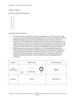
a.

Solution to Oppenheimer Visuals (25 minutes)
[Choosing the optimum technology and “all costs are variable in the long
run”]

The following table shows that Technology 2 yields the highest firm value:

Q
60
65
70
75
80
85
90
95
100
Chapter 2
2-18

Price

$760
740
720
700
680
660
640
620
600

Revenue
$45600
48100
50400
52500
54400
56100
57600
58900
60000

Technology 1
Total
cost
Profit
$46000 $-400
47000
1100
48000
2400

49000
3500
50000
4400
51000
5100
52000
5600
53000
5900
54000
6000

Technology 2
Total
cost
Profit
$40000 $5600
42000
6100
44000
6400
46000
6500
48000
6400
50000
6100
52000
5600

54000
4900
56000
4000

© McGraw-Hill Education 2017
Instructor’s Manual, Accounting for Decision Making and Control


105
110

580
560

60900
61600

55000
56000

5900
5600

58000
60000

2900
1600

b.

They should set the price at $700 per panel and sell 75 panels per day.

c.

The fixed cost of technology 2 of $16,000 per day was chosen as part of the profit
maximizing production technology. Oppenheimer could have chosen technology
1 and had a higher fixed cost and lower variable cost. But given the demand
curve the firm faces, they chose technology 2. So, at the time they selected
technology 2, the choice of fixed costs had not yet been determined and was
hence “variable” at that point in time.

P 2-27:

Solution to Eastern University Parking (25 minutes)
[Opportunity cost of land]

The University's analysis of parking ignores the opportunity cost of the land on
which the surface space or parking building sits. The $12,000 cost of an enclosed
parking space is the cost of the structure only. The $900 cost of the surface space is the
cost of the paving only. These two numbers do not include the opportunity cost of the
land which is being consumed by the parking. The land is assumed to be free. Surface
spaces appear cheaper because they consume a lot more ―free‖ land. A parking garage
allows cars to be stacked on top of each other, thereby allowing less land to be consumed.
The correct analysis would impute an opportunity cost to each potential parcel of land on
campus, and then build this cost into both the analysis and parking fees. The differential
cost of each parcel would take into account the additional walking time to the center of
campus. Remote lots would have a lower opportunity cost of land and would provide
less expensive parking spaces.

Another major problem with the University's analysis is that parking prices should
be set to allocate a scarce resource to those who value it the highest. If there is an excess
demand for parking (i.e., queues exist), then prices should be raised to manage the queue
and thereby allocate the scarce resource. Basing prices solely on costs does not guarantee
that any excess supply or demand is eliminated.
Other relevant considerations in the decision to build a parking garage include:
1.
2.

The analysis ignores the effect of poor/inconvenient parking on tuition
revenues.
Snow removal costs are likely lower, but other maintenance costs are
likely to be higher with a parking garage.

The most interesting aspect of this question is "Why have University officials
systematically overlooked the opportunity cost of the land in their decision-making
process?" One implication of past University officials’ failure to correctly analyze the
parking situation is the "dumb-administrator" hypothesis. Under this scenario, one

Chapter 2
Instructor’s Manual, Accounting for Decision Making and Control

© McGraw-Hill Education 2017
2-19


concludes that all past University presidents were ignorant of the concept of opportunity
cost and therefore failed to assign the "right" cost to the land.
The way to understand why administrators will not build a parking garage is to
ask what will happen if a garage is built and priced to recover cost. The cost of the

covered space will be in excess of $1,200 per year. Those students, faculty, and staff
with a high opportunity cost of their time (who tend to be those with higher incomes) will
opt to pay the significantly higher parking fee for the garage. Lower-paid faculty will
argue the inequity of allowing the "rich" the convenience of covered parking while the
―poor‖ are relegated to surface lots. Arguments will undoubtedly be made by some
constituents that parking spots should not be allocated using a price system which
discriminates against the poor but rather parking should be allocated based on "merit" to
be determined by a faculty committee. Presidents of universities have risen to their
positions by developing a keen sense of how faculty, students, and staff will react to
various proposals. An alternative to the "dumb-administrator" hypothesis is the "rational
self-interested administrator" hypothesis. Under this hypothesis, the parking garage is
not built because the administrators are unwilling to bear the internal political
ramifications of such a decision.
Finally, taxes play an important role in the University's decision not to build a
parking garage. If faculty are to pay the full cost of the garage, equilibrium wage rates
will have to rise to make the faculty member as well off at Eastern University paying for
parking than at another university where parking is cheaper. Because employees are
unable to deduct parking fees from their taxes, the University will have to increase
salaries by the amount of the parking fees plus the taxes on the fees to keep the faculty
indifferent about staying or leaving the University. Therefore, a parking garage paid for
by the faculty (which means paid by the University) causes the government to raise more
in taxes. The question then comes down to: is the parking garage the best use of the
University's resources?
P2-28:
a.

Solution to GRC (30 minutes)
[Choosing alternative technologies with different operating leverage]
The two technologies have different operating leverages. In order to address
which technology to choose, first compute each technology’s fixed and variable

cost. Select any two average costs from the table in the problem and solve for the
FC and VC. For Hi Automation:
$365 = FC / 5 + VC
$245 = FC / 10 + VC
120 = FC / 5 - FC / 10
1200 = 2 FC - FC
FC = $1,200
365 = 1200 / 5 + VC
365 = 240 +VC
VC = $125

Chapter 2
2-20

(definition of avg cost when Q=5)
(definition of avg cost when Q=10)
(subtract the 2nd eqn from the 1st eqn)
(multiple each side by 10)
(solve for FC)
(substitute FC=1200 into 1st eqn)

© McGraw-Hill Education 2017
Instructor’s Manual, Accounting for Decision Making and Control


Use the same approach to compute the FC and VC for Low Automation:
$295 = FC / 5 + VC
(definition of avg cost when Q=5)
$285 = FC / 10 + VC
(definition of avg cost when Q=10)

10 = FC / 5 - FC / 10
(subtract the 2nd eqn from the 1st eqn)
100 = 2 FC - FC
(multiple each side by 10)
FC = $100
(solve for FC)
295 = 100 / 5 + VC
(substitute FC=1200 into 1st eqn)
295 = 20 +VC
VC = $275
Since each technology has a different cost structure, each technology will have a
different profit maximizing price-quantity relation. To see this, the following
table computes the profits for each technology at various production levels:

Price
440
420
400
380
360
340
320
300
280
260

Quantity
3
4
5

6
7
8
9
10
11
12

Revenue
1320
1680
2000
2280
2520
2720
2880
3000
3080
3120

Total
Cost
Hi Auto
1575
1700
1825
1950
2075
2200
2325

2450
2575
2700

Profits
Hi Auto
-255
-20
175
330
445
520
555
550
505
420

Total
Cost
Low Auto
925
1200
1475
1750
2025
2300
2575
2850
3125
3400

Profits
Low Auto
395
480
525
530
495
420
305
150
-45
-280

From this table, we see that if Hi Auto is chosen, it yields a maximum profit of
$555,000 whereas if Low auto is chosen, it yields a maximum profit of $530,000.
Hi Auto yields $25,000 more profit than Low Auto. In this simplified problem
where there is no uncertainty, GRC should adopt the Hi Auto technology.
If there is substantial risk in this wind turbine venture (as there likely will be),
then GRC should consider the Lo Auto option because it lowers GRC’s fixed cost
structure, thereby reducing GRC’s operating risk. Less operating leverage, like
lower financial leverage, reduces the expected costs of financial distress.
Lowering profits by $25,000 via Low Auto may be a cheap way to reduce
operating risk.
NOTE: If the demand curve is used instead of the table, the profit maximizing
quantity for Hi Auto is 9.375 machines and 5.625 machines for Lo Auto.
At these output levels, Hi Auto yields total profits of $557,813 and Lo
Auto yields total profits of $532,813. The difference is still $25,000.

Chapter 2

Instructor’s Manual, Accounting for Decision Making and Control

© McGraw-Hill Education 2017
2-21


b.

If Hi Auto is selected, then GRC should set the price of each gear machine at
$320,000 and sell 9 machines per year. If Low Auto is selected, then GRC should
set the price of each gear machine at $380,000 and sell 6 machines per year.
NOTE: If the demand curve is used instead of the table, the profit maximizing
price for Hi Auto is $312,500 (500-20 x 9.375 machines) and $387,500
(500 - 20 x 5.625 machines) for Lo Auto.

P 2-29:

Solution to Mastich Counters (25 minutes)
[Opportunity cost to the firm of workers deferring vacation time]

At the core of this question is the opportunity cost of workers deferring vacation.
The new policy was implemented because management believed it was costing
the firm too much money when workers left with accumulated vacation and were paid.
However, these workers had given Mastich in effect a loan. By not taking their vacation
time as accrued, they stayed in their jobs and worked, allowing Mastich to increase its
output without hiring additional workers, and without reducing output or quality.
Mastich was able to produce more and higher quality output with fewer workers.
Suppose a worker is paid $20 per hour this year and $20.60 next year. By deferring one
vacation hour one year, the worker receives $20.60 when the vacation hour is taken next
year. As long as average worker salary increases are less than the firm’s cost of capital,

the firm is better off by workers accumulating vacation time. The firm receives a loan
from its workers at less than the firm’s cost of capital.
Under the new policy, and especially during the phase-in period, Mastich has
difficulty meeting production schedules and quality standards as more workers are now
on vacation at any given time. To overcome these problems, the size of the work force
will have to increase to meet the same production/quality standards. If the size of the
work force stays the same, but more vacation time is taken, output/quality will fall.
Manager A remarked that workers were refreshed after being forced to take
vacation. This is certainly an unintended benefit. But it also is a comment about how
some supervisors are managing their people. If workers are burned out, why aren’t their
supervisors detecting this and changing job assignments to prevent it? Moreover, how is
burnout going to be resolved after the phase-in period is over and workers don’t have
excess accumulated vacation time?
The new policy reduces the workers’ flexibility to accumulate vacation time,
thereby reducing the attractiveness of Mastich as an employer. Everything else equal,
workers will demand some offsetting form of compensation or else the quality of
Mastich’s work force will fall.
Many of the proposed benefits, namely reducing costs, appear illusory. The
opportunity costs of the new policy are reduced output, schedule delays, and possible
quality problems. If workers under the new policy were forfeiting a significant number
of vacation hours, these lost hours ―profit‖ the firm. But, as expected from rational
workers, very few vacation hours are being forfeited (as mentioned by Manager C).
However, there is one very real benefit of the new policy – less fraud and
embezzlement. One key indicator of fraud used by auditors is an employee who never
takes a vacation. Forced vacations mean other people have to cover the person’s job.
Chapter 2
2-22

© McGraw-Hill Education 2017
Instructor’s Manual, Accounting for Decision Making and Control

During these periods, fraud and embezzlement often are discovered. Another benefit of
this new policy is it reduces the time employees will spend lobbying their supervisors for
extended vacations (in excess of three to four weeks). Finally, under the existing policy,
employees tend to take longer average vacations (because workers have more
accumulated vacation time). When a worker takes a long vacation, it is more likely the
employee’s department will hire a temporary or ―float‖ person to fill in. With shorter
vacations, the work of the person on vacation is performed by the remaining employees.
Thus, the new policy reduces the slack (free time) of the work force and results in higher
productivity.
P 2-30:

Solution to Prestige Products (30 minutes)
[Effect of different technologies on break-even points]

a and b.
Technology
Selling price
Variable cost
Contribution margin
Fixed cost
Break-even units (fixed cost/contribution margin)
c.

German
$12.00
8.00
$4.00
$500,000

125,000

Swedish
$12.00
6.00
$6.00
$900,000
150,000

It depends. The two technologies yield identical costs at 200,000 units:
$500,000 + $8 Q = $900,000 + $6 Q
Or, Q = 200,000
So, if annual sales are expected to be above 200,000 units, Prestige should lease
the Swedish equipment and if sales are expected to be below 200,000 units
Prestige should lease the German equipment. However, even if expected annual
sales are slightly below 200,000 units, the Swedish equipment has higher capacity
and can meet sales in excess of the German machine capacity of 215,000 units.
Therefore, it is not enough to know just what expected annual sales will be, but
also its standard deviation.

d.

See below:
Technology
Expected volume
Variable cost/unit
Total variable cost
Fixed cost
Total cost
Expected volume

German
180,000
8.00
$1,440,000
500,000
$1,940,000
180,000

Chapter 2
Instructor’s Manual, Accounting for Decision Making and Control

Swedish
180,000
6.00
$1,080,000
900,000
$1,980,000
180,000
© McGraw-Hill Education 2017
2-23


Average cost

e.

$10.78

$11.00

Operating leverage is the amount of fixed costs in the firm’s cost structure. One
way to measure operating leverage is the ratio of fixed to total cost. The higher
the firm’s operating leverage, the greater the variability of the firm’s net income
to changes in volumes. Firms with little operating leverage can cut variable costs
as volume declines, and because these firms have little fixed costs, net income
remains positive. So, operating leverage affects the firm’s risk, bankruptcy
likelihood, and hence firm value.

P 2-31:

Solution to JLE Electronics (25 minutes)
[Maximize contribution margin per unit of scarce resource]

Notice that the new line has a maximum capacity of 25,200 minutes (21 ×20 ×
60) which is less than the time required to process all four orders. The profit maximizing
production schedule occurs when JLE selects those boards that have the largest
contribution margin per minute of assembly time. The following table provides the
calculations:
A
$38
23
$15

Price
Variable cost per unit
Contribution margin
Number of machine minutes
Contribution margin/minute

3
5

CUSTOMERS
B
C
$42
$45
25
27
$17
$18

D
$50
30
$20

4
4.25

6
3.33

5
3.6

Customers A, B, and C provide the highest contribution margins per minute and should
be scheduled ahead of customer D.

Number of boards requested
Number of boards scheduled to be
produced in the next 21 days

A
2500

CUSTOMERS
B
C
2300
1800

2500

2300

1700*

D
1400
0

* 1700 [25,200 – (2,500 × 3) – (2,300 × 40]/5

Chapter 2
2-24

© McGraw-Hill Education 2017
Instructor’s Manual, Accounting for Decision Making and Control