Test bank and solution of ch02 chart and graphs (1)

Student’s Solutions Manual and Study Guide: Chapter 2

Page 1

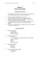
Chapter 2
Charts and Graphs
LEARNING OBJECTIVES
The overall objective of Chapter 2 is for you to master several techniques
for summarizing and depicting data, thereby enabling you to:
1.
2.

3.

4.

Construct a frequency distribution from a set of data
Construct different types of quantitative data graphs, including
histograms, frequency polygons, ogives, dot plots, and stem-and-leaf
plots, in order to interpret the data being graphed
Construct different types of qualitative data graphs, including pie charts,
bar graphs, and Pareto charts, in order to interpret the data being
graphed
Construct a cross-tabulation table and recognize basic trends in two-variable
scatter plots of numerical data.

CHAPTER OUTLINE
2.1

Frequency Distributions
Class Midpoint

Relative Frequency
Cumulative Frequency

2.2

Quantitative Data Graphs
Histograms
Using Histograms to Get an Initial Overview of the Data
Frequency Polygons
Ogives
Dot Plots
Stem and Leaf Plots

2.3

Qualitative Data Graphs
Pie Charts
Bar Graphs
Pareto Charts

2.4

Charts and Graphs for Two Variables
Cross Tabulation
Scatter Plot


Student’s Solutions Manual and Study Guide: Chapter 2

Page 2

KEY TERMS

Bar Graph
Class Mark
Class Midpoint
Cross Tabulation
Cumulative Frequency
Dot Plot
Frequency Distribution
Frequency Polygon
Grouped Data

Histogram
Ogive
Pareto Chart
Pie Chart
Range
Relative Frequency
Scatter Plot
Stem-and-Leaf Plot
Ungrouped Data

STUDY QUESTIONS

1. The following data represents the number of printer ribbons used annually in a company by
twenty-eight departments. This is an example of ______________ data.
8 4 5 10 6 5 4 6 3 4 4 6 1 12
2 11 2 5 3 2 6 7 6 12 7 1 8 9
2. Below is a frequency distribution of ages of managers with a large retail firm. This is an

example of _______________ data.
Age
20-29
30-39
40-49
50-59
over 60

f
11
32
57
43
18

3. For best results, a frequency distribution should have between _____ and _____ classes.
4. The difference between the largest and smallest numbers is called the _______________.
5. Consider the values below. In constructing a frequency distribution, the beginning point
of the lowest class should be at least as small as _____ and the endpoint of the highest
class should be at least as large as _____.
27 21 8 10 9 16 11 12 21 11 29 19 17 22 28 28 29 19 18 26 17 34 19 16 20
6. The class midpoint can be determined by _______________.


Student’s Solutions Manual and Study Guide: Chapter 2

Page 3

7-9 Examine the frequency distribution below:
class

5-under 10
10-under 15
15-under 20
20-under 25
25-under 30
30-under 35

frequency
56
43
21
11
12
8

7. The relative frequency for the class 15-under 20 is _______________.
8. The cumulative frequency for the class 20-under 25 is _______________.
9. The midpoint for the class 25-under 30 is ___________.
10. The graphical depiction that is a type of vertical bar chart and is used to depict a frequency
distribution is a _______________.
11. The graphical depiction that utilizes cumulative frequencies is a _______________.
12. The graph shown below is an example of a _______________.

13. Consider the categories below and their relative amounts:
Category
A
B
C
D
E

Amount
112
319
57
148
202

If you were to construct a Pie Chart to depict these categories, then you would allot
_______________ degrees to category D.


Student’s Solutions Manual and Study Guide: Chapter 2

Page 4

14. A graph that is especially useful for observing the overall shape of the distribution of

data points along with identifying data values or intervals for which there are
groupings and gaps in the data is called a ______________________.
15. Given the values below, construct a stem and leaf plot using two digits for the stem.
346 340 322 339 342 332 338
357 328 329 346 341 321 332
16. A vertical bar chart that displays the most common types of defects that occur with a product,
ranked in order from left to right, is called a __________________.
17. A process that produces a two-dimensional table to display the frequency counts for two
variables simultaneously is called a ____________________.
18. A two-dimensional plot of pairs of points often used to examine the relationship of two
numerical variables is called a _________________.

ANSWERS TO STUDY QUESTIONS

1. Raw or Ungrouped

11. Ogive

2. Grouped

12. Frequency Polygon

3. 5, 15

13. 148/838 of 360o = 63.6o

4. Range

14. Dot Plot

5. 8, 34

15. 32
33
34
35

6. Averaging the two class endpoints

1 2 8 9
2 2 8 9
0 1 2 6 6

7

7. 21/151 = .1391
16. Pareto Chart
8. 131
17. Cross Tabulation
9. 27.5
18. Scatter Plot
10. Histogram


Student’s Solutions Manual and Study Guide: Chapter 2

Page 5

SOLUTIONS TO THE ODD-NUMBERED PROBLEMS IN CHAPTER 2
2.1
a)

One possible 5 class frequency distribution:
Class Interval
0 - under 20
20 - under 40
40 - under 60
60 - under 80
80 - under 100

b)

One possible 10 class frequency distribution:

Class Interval
10 - under 18
18 - under 26
26 - under 34
34 - under 42
42 - under 50
50 - under 58
58 - under 66
66 - under 74
74 - under 82
82 - under 90

c)

Frequency
7
15
12
12
4
50

Frequency
7
3
5
9
7
3
6

4
4
2

The ten class frequency distribution gives a more detailed breakdown of
temperatures, pointing out the smaller frequencies for the higher temperature
intervals. The five class distribution collapses the intervals into broader
classes making it appear that there are nearly equal frequencies in each class.


Student’s Solutions Manual and Study Guide: Chapter 2

Page 6

2.3
Class
Interval
Frequency
0-5
6
5 - 10
8
10 - 15
17
15 - 20
23
20 - 25
18
25 - 30
10

30 - 35
4
TOTAL
86

Class
Midpoint
2.5
7.5
12.5
17.5
22.5
27.5
32.5

Relative
Frequency
6/86 = .0698
.0930
.1977
.2674
.2093
.1163
.0465
1.0000

Cumulative
Frequency
6
14

31
54
72
82
86

The relative frequency tells us that it is most probable that a customer is in the
15 - 20 category (.2674). Over two thirds (.6744) of the customers are between 10
and 25 years of age.

2.5

Some examples of cumulative frequencies in business:
sales for the fiscal year,
costs for the fiscal year,
spending for the fiscal year,
inventory build-up,
accumulation of workers during a hiring buildup,
production output over a time period.


Student’s Solutions Manual and Study Guide: Chapter 2

Page 7

2.7 Histogram:

Frequency Polygon:

Comment: The histogram indicates that the number of calls per shift varies widely.

However, the heavy numbers of calls per shift fall in the 50 to 80 range.
Since these numbers occur quite frequently, staffing planning should be done
with these number of calls in mind realizing from the rest of the graph that
there may be shifts with as few as 10 to 20 calls.


Student’s Solutions Manual and Study Guide: Chapter 2

2.9

STEM

Page 8

LEAF

21
22
23
24
25
26
27

2
0
0
0
0
0

0

8
1
0
0
3
1
1

8
2
4
3
4
1
3

9
4
5
6
5
2

6
8
9
5
3

6
8
9
7
3

7
9
9
7
5

9 9
9 9 9
8 9
6

Dotplot
Dotplot of Sales Prices

216

224

232

240
248
Sales Prices

256

264

272

Both the stem and leaf plot and the dot plot indicate that sales prices vary quite a bit
within the range of $212,000 and $273,000. It is more evident from the stem and
leaf plot that there is a strong grouping of prices in the five price ranges from the
$220’s through the $260’s.

2.11

The histogram shows that there are only three airports with more than 70 million
passengers. From the information given in the problem, we know that the busiest
airport is Atlanta’s Hartsfield-Jackson International Airport which has over 95
million passengers. We can tell from the graph that there is one airport with between


Student’s Solutions Manual and Study Guide: Chapter 2

Page 9

80 and 90 million passengers and another airport with between 70 and 80 million
passengers. Four airports have between 60 and 70 million passengers. Eighteen of
the top 30 airports have between 40 and 60 million passengers.

2.15

From the stem and leaf display, the original raw data can be obtained. For example,
the fewest number of cars washed on any given day are 25, 29, 29, 33, etc. The most
cars washed on any given day are 141, 144, 145, and 147. The modal stems are 3, 4,
and 10 in which there are 6 days with each of these numbers. Studying the left
column of the Minitab output, it is evident that the median number of cars washed is
81. There are only two days in which 90 some cars are washed (90 and 95) and only
two days in which 130 some cars are washed (133 and 137).

Firm
Intel Corp.
Texas Instruments
Qualcomm
Micron Technology
Broadcom
TOTAL

Proportion
.5624
.1594
.1141
.0831
.0810
1.0000

Degrees
202.5
57.4
41.1
29.9
29.2

360.1

a.) Bar Graph:
Bar Chart - Problem 2.15 a
50000

40000

Revenue

2.13

30000

20000

10000

0

Intel Corp

b.) Pie Chart:

Texas Instr.

Qualcomm
Firm

Micron Tech.

Broadcom


Student’s Solutions Manual and Study Guide: Chapter 2

Page 10

Pie Chart of Revenue - Problem 2.15 b
Broadcom
7153, 8.1%
Micron Tech.
7344, 8.3%

Qualcomm
10080, 11.4%

Intel Corp
49685, 56.2%

Texas Instr.
14081, 15.9%

c.) While pie charts are sometimes interesting and familiar to observe, in this
problem it is virtually impossible from the pie chart to determine the
relative difference between Micron Technology and Broadcom. In fact, it
is somewhat difficult to judge the size of Qualcomm and Texas
Instruments. From the bar chart, however, relative size is easier to judge,
especially the difference between Qualcomm and Texas Instruments.

Student’s Solutions Manual and Study Guide: Chapter 2

Brand
Johnson & Johnson
Pfizer
Abbott Laboratories
Merck
Eli Lilly
Bristol-Myers Squibb
TOTAL

Proportion
.294
.237
.146
.130
.104
.089
1.000

Degrees
106
85
53
47
37
32
360

Pie Chart:
Pharmaceutical Sales
Bristol-My ers Squibb
8.9%
Eli Lilly
10.4%

Johnson & Johnson
29.4%

Merck
13.0%

Abbott Laboratories
14.6%

Pfizer
23.7%

Bar Graph:
Bar Chart of Sales
70000
60000
50000

Sales

2.17

Page 11

40000
30000
20000
10000
0

Johnson & Johnson

Pfizer

Abbott Laboratories

Merck

Pharmaceutical Company

Eli Lilly

Bristol-Myers Squibb


Student’s Solutions Manual and Study Guide: Chapter 2

Complaint
Busy Signal
Too long a Wait
Could not get through
Got Disconnected
Transferred to the Wrong Person

Poor Connection
Total

Number
420
184
85
37
10
8
744

% of Total
56.45
24.73
11.42
4.97
1.34
1.08
99.99

Customer Complaints
800
700
600
500
400
300
200
100

0

100
80
60
40
20

C1

sy
Bu

l
na
si g
o
To

d
ul
Co
Count
Percent
Cum %

420
56.5
56.5

ng
lo

a

e
tg
no

w

t
ai

hr
tt

gh
ou

to

an

t
en
ag

o
sc

di
t
Go

Tr
184
24.7
81.2

s
an

85
11.4
92.6

e
nn

ed
rr
fe

ed
ct

to

e
th

w

37
5.0
97.6

ng
ro

pe

on
rs
o
Po

10
1.3
98.9

n
io
ct
e
n
on
c
r

8
1.1
100.0

0

Percent

Count

2.19

Page 12


Student’s Solutions Manual and Study Guide: Chapter 2

Page 13

Sales

2.21

Advertising

Generally, as advertising dollars increase, sales are increasing.

2.23 There is a slight tendency for there to be a few more absences as plant workers
Commute further distances. However, compared to the total number of workers in
each category, these increases are relatively small (2.5% to 3.0% to 6.6%).

Comparing workers who travel 4-10 miles to those who travel 0-3 miles, there is
about a 2:1 ratio in all three cells indicating that for these two categories
(0-3 and 4-10), number of absences is essentially independent of commute distance.

2.25

Class Interval

Frequencies

16 - under 23
23 - under 30
30 - under 37
37 - under 44
44 - under 51
51 - under 58
TOTAL

6
9
4
4
4
3
30


Student’s Solutions Manual and Study Guide: Chapter 2

2.27

Page 14

Class Interval

Frequencies

50 - under 60
60 - under 70
70 - under 80
80 - under 90
90 - under 100
TOTAL

13
27
43
31
9
123

Histogram:

Frequency Polygon:


Student’s Solutions Manual and Study Guide: Chapter 2

Ogive:

2.29

STEM
28
29
30
31
32
33

LEAF
4
0
1
1
4
5

6
4
6
2
4

9
8
8 9
4 6 7 7
6

Page 15


Student’s Solutions Manual and Study Guide: Chapter 2

2.31

Page 16

Bar Graph:
Category
A
B
C
D
E

Frequency
7
12
14
5
19

20

Frequency

15

10

5

0

A

B

C
Category

D

2.33 Scatter Plot
16
14
12
10
y

8
6
4
2
0
0

5

10
x

15

20

E


Student’s Solutions Manual and Study Guide: Chapter 2

Page 17

2.35
Class
Interval
20 – 25
25 – 30
30 – 35
35 – 40
40 – 45
45 – 50
TOTAL

2.37

Frequency
8

6
5
12
15
7
53

Class
Midpoint
22.5
27.5
32.5
37.5
42.5
47.5

Relative
Frequency
8/53 = .1509
.1132
.0943
.2264
.2830
.1321
.9999

Frequency Distribution:
Class Interval
10 - under 20
20 - under 30

30 - under 40
40 - under 50
50 - under 60
60 - under 70
70 - under 80
80 - under 90

Histogram:

Frequency
2
3
9
7
12
9
6
2
50

Cumulative
Frequency
8
14
19
31
46
53

Student’s Solutions Manual and Study Guide: Chapter 2

Page 18

Frequency Polygon:
14
F
12
r
e 10
q 8
u 6
e
4
n
2
c
y 0
10

20

30

40

50

60

70

80

90

Class Endpoints

The normal distribution appears to peak near the center and diminish towards the
end intervals.

2.39

a.) Stem and Leaf Plot
STEM
1
2
3

LEAF
2, 3, 6, 7, 8, 8, 8, 9, 9
0, 3, 4, 5, 6, 7, 8
0, 1, 2, 2

b.) Dot Plot
Dotplot

12

15

18

21
24
Travel Time in Days

27

30


Student’s Solutions Manual and Study Guide: Chapter 2

Page 19

c.) Comments:
Both the dot plot and the stem and leaf plot show that the travel times are
relatively evenly spread out between 12 days and 32 days. The stem and leaf
plot shows that the most travel times fall in the 12 to 19 day interval followed
by the 20 to 28 day interval. Only four of the travel times were thirty or more
days. The dot plot show that 18 days is the most frequently occurring travel
time (occurred three times).

2.41
Price
$1.75 - under $1.90
$1.90 - under $2.05
$2.05 - under $2.20
$2.20 - under $2.35

$2.35 - under $2.50
$2.50 - under $2.65
$2.65 - under $2.80

Histogram:

Frequency
9
14
17
16
18
8
5
87

Cumulative
Frequency
9
23
40
56
74
82
87


Student’s Solutions Manual and Study Guide: Chapter 2

Page 20

Frequency Polygon:

20
F
r 15
e
q
10
u
e
5
n
c
0
y

1.75

1.9

2.05

2.2

2.35

2.5

2.65

2.8

2.65

2.8

Price of Sugar ($)

Ogive:

C
u
m
u
l
a
t
i
v
e

F
r
e
q
u
e
n
c

y

100
90
80
70
60
50
40
30
20
10
0
1.75

1.9

2.05

2.2

2.35

Price of Sugar ($)

2.5


Student’s Solutions Manual and Study Guide: Chapter 2

Page 21

Manufactured Goods ($ billions)

2.43

700
600
500
400
300
200
100
0
0

5

10

15

20

25

30

35

Agricultural Products ($ billions)

It can be observed that as the U.S. import of agricultural products increased, the
U.S. import of manufactured goods also increased. As a matter of fact, a nonlinear association may exist between the two variables.


Student’s Solutions Manual and Study Guide: Chapter 2

Page 22

2.45

500

100

400

80

300

60

200

40

100

20

0

C1
Count
Percent
Cum %

Fault in plastic
221
44.2
44.2

Thickness Broken handle
117
86
23.4
17.2
67.6
84.8

Labeling
44
8.8
93.6

Discoloration
32
6.4

100.0

Percent

Count

Causes of Poor Quality Bottles

0

One of the main purposes of a Pareto chart is that it has the potential to help
prioritize quality initiatives by ranking the top problems in order starting with
the most frequently occurring problem. Thus, all things being equal, in
attempting to improve the quality of plastic bottles, a quality team would begin
with studying why there is a fault in plastic and determining how to correct for
it. Next, the quality team would study thickness issues followed by causes of
broken handles. Assuming that each problem takes a comparable time and effort
to solve, the quality team could make greater strides sooner by following the
items shown in the Pareto chart from left to right.


Student’s Solutions Manual and Study Guide: Chapter 2

Page 23

2.47 The distribution of household income is bell-shaped with an average of about
$ 90,000 and a range of from $ 30,000 to $ 140,000.

2.49 Family practice is the most prevalent specialty with about 20% of physicians being
in family practice and pediatrics next at slightly less that. A virtual tie exists

between ob/gyn, general surgery, anesthesiology, and psychiatry at about 14% each.

2.51 There appears to be a relatively strong positive relationship between the
NASDAQ-100 and the DJIA. Note that as the DJIA became higher, the
NASDAQ-100 tended to also get higher. The slope of the graph was steeper for
lower values of the DJIA and for higher values of the DJIA. However, in the
middle, when the DJIA was from about 8600 to about 10,500, the slope was
considerable less indicating that over this interval as the DJIA rose, the
NASDAQ-100 did not increase as fast as it did over other intervals.