Điện tử viễn thông ch20 khotailieu

Mark Fritz, et. al.. "Mass and Weight Measurement."
Copyright 2000 CRC Press LLC. <>.


Mass and Weight
Measurement
Mark Fritz
Denver Instrument Company

Emil Hazarian
Denver Instrument Company

20.1
20.2

Weighing Instruments
Weighing Techniques

Mass and weight are often used interchangeably; however, they are different. Mass is a quantitative
measure of inertia of a body at rest. As a physical quantity, mass is the product of density and volume.
Weight or weight force is the force with which a body is attracted toward the Earth. Weight force is
determined by the product of the mass and the acceleration of gravity.

M =V × D

(20.1)

where M = mass
V = volume
D = density
Note: In most books, the symbol for density is the Greek letter ρ.

W =M ×G

(20.2)

where W = weight
G = gravity
The embodiment of units of mass are called weights; this increases the confusion between mass and
weight. In the International System of Units (SI), the modernized metric measurement system, the unit
for mass is called the kilogram and the unit for force is called the newton. In the United States, the
customary system the unit for mass is called the slug and the unit for force is called the pound. When
using the U.S. customary units of measure, people are using the unit pound to designate the mass of an
object because, in the United States, the pound has been defined in terms of the kilogram since 1893.

20.1 Weighing Instruments
Weighing is one of the oldest known measurements, dating back to before written history. The equal
arm balance was probably the first instrument used for weighing. It is a simple device in which two pans
are suspended from a beam equal distance from a central pivot point. The standard is placed in one pan
and the object to be measured is placed in the second pan; when the beam is level, the unknown is equal
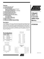
to the standard. This method of measurement is still in wide use throughout the world today. Figure 20.1
shows an Ainsworth equal arm balance.

© 1999 by CRC Press LLC


FIGURE 20.1 Ainsworth FV series equal arm balance. (Courtesy Denver Instrument Company.)

A balance is a measuring instrument used to determine the mass of an object by measuring the force
exerted by the object on its support within the gravitational field of the Earth. One places a standard of
known value on one pan of the balance. One then adds the unknown material to the second pan, until

the gravitational force on the unknown material equals the gravitational force on the standard. This can
be expressed mathematically as:

S × G =U × G

(20.3)

where S = mass of the standard
G = gravity
U = mass of the unknown
Given the short distance between pans, one assumes that the gravitational forces acting on them are
equal. Another assumption is that the two arms of the balance are equal.
Since the gravitational force is equal, it can be removed from the equation and the standard and the
unknown are said to be equal. This leads to one of the characteristics of the equal arm balance as well
as of other weighing devices, the requirement to have a set of standards that allows for every possible
measured value. The balance can only indicate if objects are equal and has a limited capability to determine
how much difference there is between two objects.
© 1999 by CRC Press LLC


Probably, the first attempt to produce direct reading balances was the introduction of the single pan
substitution balance. A substitution balance is, in principle, similar to an equal arm balance. The object
to be measured is placed in the weighing pan; inside the balance are a series of calibrated weights that
can be added to the standard side of the balance, through the use of dials and levers. The standard weights
can be added and subtracted through the use of the balance’s mechanical system, to equal a large variety
of weighing loads. Very small differences between the standard weights and the load are read out on an
optical scale.
The spring scale is probably the least expensive device for making mass measurements. The force of
gravity is once again used as the reference. The scale is placed so that the unknown object is suspended
by the spring and the force of gravity can freely act on the object. The elasticity of the spring is assumed

to be linear and the force required to stretch it is marked on the scale. When the force of gravity and the
elastic force of the spring balance, the force is read from the scale, which has been calibrated in units of
mass. Capacity can be increased by increasing the strength of the spring. However, as the strength of the
spring increases, the resolution of the scale decreases. This decrease in resolution limits spring scales to
relatively small loads of no more than a few kilograms. There are two kinds of springs used: spiral and
cantilevered springs.
The torsion balance is a precise adaptation of the spring concept used to determine the mass indirectly.
The vertical force produced by the load produces a torque on a wire or beam. This torque produces an
angular deflection. As long as the balance is operated in the linear range, the angular deflection is
proportional to the torque. Therefore, the angular deflection is also proportional to the applied load.
When the torsion spring constant is calibrated, the angular deflection can be read as a mass unit. Unlike
the crude spring scales, it is possible to make torsion balances capable of measuring in the microgram
region. The torsion element could be a band, a wire, or a string.
The beam balance is probably the next step in accuracy and cost. The beam balance uses the same
principle of operation as the equal arm balance. However, it normally has only one pan and the beam
is offset. A set of sliding weights are mounted on the beam. As the weights slide out the beam, they gain
a mechanical advantage due to the inequality of the distance from the pivot point of the balance. The
weights move out along the beam until the balance is in equilibrium. Along the beam, there are notched
positions that are marked to correspond to the force applied by the sliding weights. By adding up the
forces indicated by the position of each weight, the mass of the unknown material is determined. Beam
balances and scales are available in a wide range of accuracy’s load capacities. Beam balances are available
to measure in the milligram range and large beam scales are made with capacities to weigh trucks and
trains. Once again, the disadvantage is that as load increases the resolution decreases. Figure 20.2 shows
an example of a two pan beam balance.
The next progression in cost and accuracy is the strain gage load cell. A strain gage is an electrically
resistive wire element that changes resistance when the length of the wire element changes. The gage is
bonded to a steel cylinder that will shorten when compressed or lengthen when stretched. Because the
gage is bonded to the cylinder, the length of the wire will lengthen or contract with the cylinder. The
electrical resistance is proportional to the length of the wire element of the gage. By measuring the
resistance of the strain gage, it is possible to determine the load on the load cell. The electric resistance

is converted into a mass unit readout by the electric circuitry in the readout device.
The force restorative load cell is the heart of an electronic balance, shown in Figure 20.3. The force
restorative load cell uses the principle of the equal arm balance. However, in most cases, the fulcrum is
offset so it is no longer an equal arm balance, as one side is designed to have a mechanical advantage.
This side of the balance is attached to an electric coil. The coil is suspended in a magnetic field. The
other side is still connected to a weighing pan. Attached to the beam is a null indicating device, consisting
of a photodiode and a light-emitting diode (LED) that are used to determine when the balance is in
equilibrium. When a load is placed on the weighing pan, the balance goes out of equilibrium. The LED
photodiode circuit detects that the balance is no longer in equilibrium, and the electric current in the
coil is increased to bring the balance back to equilibrium. The electric current is then measured across
a precision sense resistor and converted into a mass unit reading and displayed on the digital readout.

© 1999 by CRC Press LLC


FIGURE 20.2 Beam balance. (Courtesy Denver Instrument Company.)

FIGURE 20.3 Force restorative load cell. (Courtesy Denver Instrument Company.)

A variation of the latter is the new generation of industrial scales, laboratory balances, and mass comparators. Mass comparators are no longer called balances because they always perform a comparison
between known masses (standards) and unknown masses. These weighing devices are employing the
electromagnetic force compensation principle in conjunction with joint flexures elements replacing the

© 1999 by CRC Press LLC


traditional knife-edge joints. Some of the advantages include a computer interfacing capability and a
maintenance-free feature because there are no moving parts.
Another measuring method used in the weighing technology is the vibrating cord. A wire or cord of
known length, which vibrates transversely, is tensioned by the force F. The vibration frequency changes

in direct proportion to the load F. The piezoelectric effect is also used in weighing technology. Such
weighing devices consist of the presence of an electric voltage at the surface of a crystal when the crystal
is under load. Balances employing the gyroscopic effect are also used. This measuring device uses the
output signal of a gyrodynamic cell similar to the frequency. Balances wherein the weight force of the
load changes the reference distance of the capacitive or inductive converters are also known. As well,
balances using the radioactivity changes of a body as a function of its mass under certain conditions exist.

20.2 Weighing Techniques
When relatively low orders of accuracy are required, reading mass or weight values directly from the
weighing instrument are adequate. Except for the equal arm balance and some torsion balances, most
modern weighing instruments have direct readout capability. For most commercial transactions and for
simple scientific experiments, this direct readout will provide acceptable results.
In the case of equal arm balances, the balance will have a pointer and a scale. When relatively low
accuracy is needed, the pointer and scale are used to indicate when the balance is close to equilibrium.
The same is true when using a torsion balance. However, the equal arm balances of smaller (e.g., 30 g)
or larger (e.g., 900 kg) capacity are also used for high-accuracy applications. Only the new generation of
electronic balances are equal or better in terms of accuracy and benefit from other features.
Weighing is a deceptively simple process. Most people have been making and using weighing measurements for most of their lives. We have all gone to the market and purchased food that is priced by
weight. We have weighed ourselves many times, and most of us have made weight or mass measurements
in school. What could be simpler? One places an object on the weighing pan or platform and reads the
result.
Unfortunately, the weighing process is very susceptible to error. There are errors caused by imperfections in the weighing instrument; errors caused by biases in the standards used; errors caused by the
weighing method; errors caused by the operator; and errors caused by environmental factors. In the case
of the equal arm balance, any difference between the lengths of the arms will result in a bias in the
measurement result. Nearly all weighing devices will have some degree of error caused by small amounts
of nonlinearity in the device. All standards have some amount of bias and uncertainty. Mass is the only
base quantity in the International System of Units (SI) defined in relation with a physical artifact. The
international prototype of the kilogram is kept at Sevres in France, under the custody of the International
Bureau of Weights and Measures. All weighing measurements originate from this international standard.
The international prototype of the kilogram is, by international agreement, exact; however, over the last

century, it has changed in value. What one does not know is the exact magnitude or direction of the
change. Finally, environmental factors such as temperature, barometric pressure, and humidity can affect
the weighing process.
There are many weighing techniques used to reduce the errors in the weighing process. The simplest
technique is substitution weighing. The substitution technique is used to eliminate some of the errors
introduced by the weighing device. The single-substitution technique is one where a known standard
and an unknown object are both weighed on the same device. The weighing device is only used to
determine the difference between the standard and the unknown. First, the standard is weighed and the
weighing device’s indication is noted. (In the case of an equal arm balance, tare weights are added to the
second pan to bring the balance to equilibrium.) The standard is then removed from the weighing device
and the unknown is placed in the same position. Again, the weighing device’s indication is noted. The
first noted indication is subtracted from the second indication. This gives the difference between the
standard and the unknown. The difference is then added to the known value of the standard to calculate
the value of the unknown object. A variation of this technique is to use a small weight of known value
© 1999 by CRC Press LLC


to offset the weighing device by a small amount. The amount of offset is then divided by the known
value of the small weight to calibrate the readout of the weighing device. The weighing results of this
measurement is calculated as follows:

(

)( ) (O − O )

U = S + O2 − O1 SW
where U
S
SW
O1

O2
O3

3

(20.4)

2

= value of the unknown
= known value of the standard
= small sensitivity weight used to calibrate the scale divisions
= first observation (standard)
= second observation (unknown)
= third observation (unknown + SW)

These techniques remove most of the errors introduced by the weighing device, and are adequate when
results to a few tenths of a gram are considered acceptable.
If results better than a few tenths of a gram are required, environmental factors begin to cause
significant errors in the weighing process. Differences in density between the standard and the unknown
object and air density combine together to cause significant errors in the weighing process.
It is the buoyant force that generates the confusion in weighing. What is called the “true mass” of an
object is the mass determined in vacuum. The terms “true mass” and “mass in vacuum” are referring to
the same notion of inertial mass or mass in the Newtonian sense. In practical life, the measurements are
performed in the surrounding air environment. Therefore, the objects participating in the measurement
process adhere to the Archimedean principle being lifted with a force equal to the weight of the displaced
volume of air. Applying the buoyancy correction to the measurement requires the introduction of the
term “apparent mass.” The “apparent mass” of an object is defined in terms of “normal temperature”
and “normal air density,” conventionally chosen as 20°C and 1.2 mg cm–3, respectively. Because of these
conventional values, the “apparent mass” is also called the “conventional mass.” The reference material

is either brass (8.4 g cm–3) or stainless steel (8.0 g cm–3), for which one obtains an “apparent mass versus
brass” and an “apparent mass versus stainless steel,” respectively. The latter is preferred for reporting the
“apparent mass” of an object.
Calibration reports from the National Institute of Standards and Technology will report mass in three
ways: True Mass, Apparent Mass versus Brass, and Apparent Mass versus Stainless Steel. Conventional
mass is defined as the mass of an object with a density of 8.0 g cm–3, at 20°C, in air with a density of
1.2 mg cm–3. However, most scientific weighings are of materials with densities that are different from
8.0 g cm–3. This results in significant measurement errors.
As an example, use the case of a chemist weighing 1 liter of water. The chemist will first weigh a mass
standard, a 1 kg weight made of stainless steel; then the chemist will weigh the water. The 1 kg mass
standard made of 8.0 g cm–3 stainless steel will have a volume of 125 cm3. The same mass of water will
have a volume approximately equal to 1000 cm3 (Volume = Mass/Density). The mass standard will
displace 125 cm3 of air, which will exert a buoyant force of 150 mg (125 cm3 × 1.2 mg cm–3). However,
the water will displace 1000 cm3 air, which will exert a buoyant force of 1200 mg (1000 cm3 × 1.2 mg cm–3).
Thus, the chemist has introduced a significant error into the measurement by not taking the differing
densities and air buoyancy into consideration.
Using 1.2 mg cm–3 for the density of air is adequate for measurements made close to sea level; it must
be noted that air density decreases with altitude. For example, the air density in Denver, CO, is approximately 0.98 mg cm–3. Therefore, to make accurate mass measurements, one must measure the air density
at the time of the measurement if environmental errors in the measurement are to be reduced.
Air density can be calculated to an acceptable value using the following equations:

(

)(

ρA ≅ 0.0034848 t + 273.15 P − 0.0037960 × U × es

© 1999 by CRC Press LLC

)

(20.5)


where ρA
t
P
U
es

= air density in mg cm–3
= temperature in °C
= barometric pressure in pascals
= relative humidity in percent
= saturation vapor pressure

(

)

es ≅ 1.7526 × 1011 × e

( −5315.56 (273.15 + t ))

(20.6)

where e ≅ 2.7182818
t = temperature in °C
To apply an air buoyancy correction to the single substitution technique, use the following formulae:

(

)(

) (

(

M u =  M s 1 − ρA ρs + O2 − O1 M SW 1 − ρA ρSW
where Mu
Ms
Msw
ρA
ρs
ρu
ρsw
O1
O2
O3

) (O − O )) (1 − ρ
3

2

A

ρu

)

(20.7)

= mass of the unknown (in a vacuum)
= mass of the standard (in a vacuum)
= mass of the sensitivity weight
= air density
= density of the standard
= density of the unknown
= density of the sensitivity weight
= first observation (standard)
= second observation (unknown)
= third observation (unknown + SW)

(

CM = M u 1 − 0.0012 ρu

) 0.99985

(20.8)

where CM = conventional mass
Mu = mass of the unknown in a vacuum
ρu = density of the unknown
When very precise measurements are needed, the double-substitution technique coupled with an air
buoyancy correction will provide acceptable results for nearly all scientific applications. The doublesubstitution technique is similar to the single-substitution technique using the sensitivity weight. In the
double-substitution technique, the sensitivity weight is weighed with both the mass standard and the
unknown. The main advantage of this technique over single substitution is that any drift in the weighing
device is accounted for in the technique. Because of the precision of this weighing technique, it is only

appropriate to use it on precision balances or mass comparators. As in the case of single substitution,
one places the standard on the balance pan and takes a reading. The standard is then removed and the
unknown object is placed on the balance pan and a second reading is taken. The third step is to add the
small sensitivity weight to the pan with the unknown object and take a third reading. Then remove the
unknown object and return the standard to the pan with the sensitivity weight and take a fourth reading.
The mass is calculated using the following formulae:

Mu =

© 1999 by CRC Press LLC

(M (1 − ρ ρ ) + (O − O + O − O )) 2 (M ( 1 − ρ
S

A

S

2

1

3

4

(1 − ρ

A

ρu

)

SW

A

ρSW

) (O − O ))
3

2

(20.9)


where Mu
Ms
Msw
ρA
ρs
ρu
ρsw
O1
O2
O3
O4

= mass of the unknown (in a vacuum)
= mass of the standard (in a vacuum)
= mass of the sensitivity weight
= air density
= density of the standard
= density of the unknown
= density of the sensitivity weight
= first observation (standard)
= second observation (unknown)
= third observation (unknown + sensitivity weight)
= fourth observation (standard + sensitivity weight)

(

CM = M u 1 − 0.0012 ρu

) 0.99985

(20.10)

where CM = conventional mass
Mu = mass of the unknown in a vacuum
ρu = density of the unknown
To achieve the highest levels of accuracy, advanced weighing designs have been developed. These
advanced weighing designs incorporate redundant weighing, drift compensation, statistical checks, and
multiple standards. The simplest of these designs is the three-in-one design. It uses two standards to
calibrate one unknown weight. In its simplest form, one would perform three double substitutions. The
first compares the first standard and the unknown weight; the second double substitution compares the
first standard against the second standard, which is called the check standard; and the third and final
comparison compares the second (or check standard) against the unknown weight. These comparisons

would then result in the following:
O1
O2
O3
O4
O5
O6
O7
O8
O9
O10
O11
O12

= reading with standard on the balance
= reading with unknown on the balance
= reading with unknown and sensitivity weight on the balance
= reading with standard and sensitivity weight on the balance
= reading with standard on the balance
= reading with check standard on the balance
= reading with check standard and sensitivity weight on the balance
= reading with standard and sensitivity weight on the balance
= reading with check standard on the balance
= reading with unknown on the balance
= reading with unknown and sensitivity weight on the balance
= reading with check standard and sensitivity weight on the balance

The measured differences are calculated using the following formulae:

[(

) ] [

[(

) 2] × [M (1 − ρ

(

a = O1 − O2 + O4 − O3 2 × M SW 1 − ρA ρSW
b = O5 − O6 + O8 − O7

[(

SW

) ] [

(

A

ρSW

c = O9 − O10 + O12 − O11 2 × M SW 1 − ρA ρSW

© 1999 by CRC Press LLC

) O −O ]

(20.11)

) O −O ]

(20.12)

3

7

)O

11

2

6

− O10

]

(20.13)


where a
b
c
Msw
ρA

ρsw

= difference between standard and unknown
= difference between standard and check standard
= difference between check standard and unknown
= mass of sensitivity weight
= air density calculated using Equations 20.5 and 20.6
= density of sensitivity weight

The least-squares measured difference is computed for the unknown from:

(

)

du = −2a − b − c 3

(20.14)

Using the least-squares measured difference, the mass of the unknown is computed as:

((

) ) (1 − ρ

U = S 1 − ρA ρS + du

A

ρU

)

(20.15)

where U = mass of unknown
S = mass of the standard
du = least-squares measured difference of the unknown
ρA = air density calculated using Equations 20.5 and 20.6
ρS = density of the standard
ρU = density of the unknown
The conventional mass of the unknown is now calculated as:

(

CU = U 1 − 0.0012 ρU

) 0.99985

(20.16)

where CU = conventional mass
U = mass of unknown
ρU = density of unknown
The least-squares measured difference is now computed for the check standard as:

(

)

dCS = −a − 2b − c 3

(20.17)

Using the least-squares measured difference, the mass of the check standard is computed from:

((

)

CS = S 1 − ρA ρS + dCS
where CS
s
dCS
ρA
ρS
ρCS

) (1 − ρ

A

ρCS

)

(20.18)

= mass of check standard
= mass of the standard

= least-squares measured difference of the check standard
= air density calculated using Equations 20.5 and 20.6
= density of the standard
= density of unknown

The mass of the check standard must lie within the control limits for the check standard. If it is out of
the control limits, the measurement must be repeated.
The short-term standard deviation of the process is now computed:

(

Short-term standard deviation = 0.577 a − b + c

© 1999 by CRC Press LLC

)

(20.19)


The short-term standard deviation is divided by the historical pooled short-time standard deviation
to calculate the F-statistic:

F-statistic = short-term standard deviation/pooled short-time standard deviation
The F-statistic must be less than the value obtained from the student t-variant at the 99% confidence
level for the number of degrees of freedom of the historical pooled standard deviation. If this test fails,
the measurement is considered to be out of statistical control and must be repeated.
By measuring a check standard and by computing the short-term standard deviation of the process
and comparing them to historical results, one obtains a high level of confidence in the computed value
of the unknown.

There are many different weighing designs that are valid; the three-in-one (three equal weights) and
four equal weights are the ones that can be easily calculated without the use of a computer. Primary
calibration laboratories — private and government — are using these multiple intercomparisons, stateof-the-art mass calibration methods under the Mass Measurement Assurance Program using the Mass
Code computer program provided by the National Institute of Standards and Technology. A full discussion of these designs can be found in the National Bureau of Standards Technical Note 952.

References
1. J. K. Taylor and H. V. Oppermann, Handbook for the Quality Assurance of Metrological Measurements, NBS Handbook 145, Washington, D.C.: U.S. Department of Commerce, National Bureau
of Standards, 1986.
2. L. V. Judson, Weights and Measures Standards of the United States, A Brief History, NBS Special
Publication 447, Washington, D.C.: Department of Commerce, National Bureau of Standards, 1976.
3. P. E. Pontius, Mass and Mass Values, NBS Monograph 133, Washington, D.C.: Department of
Commerce, National Bureau of Standards, 1974.
4. K.B. Jaeger and R. S. Davis, A Primer for Mass Metrology, NBS Special Publication 700-1, Washington, D.C.: Department of Commerce, National Bureau of Standards, 1984.
5. J. M. Cameron, M. C. Croarkin, and R. C. Raybold, Designs for the Calibration of Standards of
Mass, NBS Technical Note 952, Washington, D.C.: Department of Commerce, National Bureau of
Standards, 1977.
6. G. L. Harris (Ed.), Selective Publications for the Advanced Mass Measurements Workshop, NISTIR
4941, Washington, D.C.: Department of Commerce, National Institute of Standards and Technology, 1992.
7. Metron Corporation, Physical Measurements, NAVAIR 17-35QAL-2, California: U.S. Navy, 1976.
8. R. S. Cohen, Physical Science, New York: Holt, Rinehart and Winston, 1976.
9. D. B. Prowse, The Calibration of Balances, CSIRO Division of Applied Physics, Australia, 1995.
10. E. Hazarian, Techniques of mass measurement, Southern California Edison Mass Seminar Notebook,
Los Angeles, CA, 1994.
11. E. Hazarian, Analysis of mechanical convertors of electronic balances, Measurement Sci. Conf.,
Anaheim, CA, 1993.
12. B. N. Taylor, Guide for the use of the International System of Units (SI), NIST SP811, 1995.

© 1999 by CRC Press LLC