Điện tử viễn thông teletrafic khotailieu

Contents
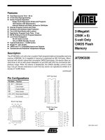
Feature
Guest editorial, Arne Myskja ............................... 1

Testing ATM switches, Sveinung O Groven ... 147

An introduction to teletraffic, Arne Myskja ......... 3

The effect of end system hardware and
software on TCP/IP throughput performance
over a local ATM network, Kjersti Moldeklev,
Espen Klovning, Øivind Kure........................... 155

A tribute to A.K. Erlang, Arne Myskja .............. 41
The life and work of Conny Palm
– some personal comments and experiences,
Rolf B Haugen ................................................... 50
Architectures for the modelling of QoS
functionality, Finn Arve Aagesen ...................... 56
Observed traffic variations and their influence
in choice of intensity measurement routine,
Asko Parviala .................................................... 69
Point-to-point losses in hierarchical alternative
routing, Bengt Wallström ................................... 79
On overload control of SPC-systems,
Ulf Körner ......................................................... 82
Capacity of an Alcatel 1000 S12 exchange
emphasised on the ISDN remote subscriber unit,
John Ytterhaug, Gunnar Nossum,
Rolv-Erik Spilling .............................................. 87

Structure and principles of Telenor’s
ISDN/PSTN target network, Arne Østlie .......... 95
Teletraffic analysis of mobile communications
systems, Terje Jensen ...................................... 103
Analysis of external traffic at UNIT/SINTEF’s
MD110 telephone exchange,
Boning Feng, Arne Myskja .............................. 119

Investigations on Usage Parameter Control and
Connection Admission Control in the EXPLOIT
testbed, Egil Aarstad, Johannes Kroeze,
Harald Pettersen, Thomas Renger .................. 168
Synthetic load generation for ATM traffic
measurements, Bjarne E Helvik ...................... 174
Speed-up techniques for high-performance
evaluation, Poul E Heegaard .......................... 195
Some important models for ATM,
Olav Østerbø ................................................... 208
Notes on a theorem of L. Takács on single
server queues with feedback, Eliot J Jensen ... 220

Status
International research and standardization
activities in telecommunication: Introduction,
Endre Skolt ...................................................... 225
Document types that are prepared by ETSI,
Trond Ulseth .................................................... 226
ATM traffic activities in some RACE projects,
Harald Pettersen ............................................. 229

LAN Interconnection Traffic Measurements,
Sigmund Gaaren .............................................. 130

The PNO Cipher project, Øyvind Eilertsen ..... 232

Aspects of dimensioning transmission resources
in B-ISDN networks, Inge Svinnset ................. 139

A presentation of the authors ........................... 235

Telektronikk
Volume 91 No. 2/3 - 1995
ISSN 0085-7130

Editorial office:
Telektronikk
Telenor AS, Telenor Research & Development
P.O. Box 83
N-2007 Kjeller, Norway

Editor:
Ola Espvik
Tel. + 47 63 84 88 83

Editorial board:
Ole P Håkonsen, Senior Executive Vice President
Karl Klingsheim, Vice President, Research
Bjørn Løken, Vice President, Market and Product Strategies

Status section editor:

Endre Skolt
Tel. + 47 63 84 87 11

Graphic design:
Design Consult AS

Editorial assistant:
Gunhild Luke
Tel. + 47 63 84 86 52

Layout and illustrations:
Gunhild Luke, Britt Kjus, Åse Aardal
Telenor Research & Development


Guest editorial
BY ARNE MYSKJA

The situation is familiar: Some
nice, new communication system
with fancy facilities is installed,
and everybody is happy. Until
some day the system response
gets slow, or blocking occurs
more and more frequently. Something must be done, but what? In
a simple network it may be a
straightforward matter of adding
capacity, even though on the way
costly time is wasted. In the more
complicated systems diagnosis is

also more difficult. One may have
to do systematic observations and
carry out sophisticated analyses.
The problem is no longer that of
correct operation in accordance
with the functional design of the
system. It is rather a matter of
how to give service to many
uncoordinated users simultaneously by means of a system
with limited capacity.
With the extremely large and
complicated telecommunications
networks of today two main considerations may be pointed out: functionality and quality. An
important subset of quality characteristics is that of traffic performance. A functionally good solution may at times be rather
useless if the traffic dimensioning and control are inadequate. In
this issue of “Telektronikk” teletraffic is chosen as the theme in
focus.
In the early days of telephony – around the last turn of the century – users encountered blocking and waiting situations because of shared subscriber lines, inadequate switchboard or
operator capacity, or busy or unavailable called users. Later,
trunk lines between switchboards became a concern, and the
introduction of automatic switches – for all their advantages –
stripped the network of intelligent information and control functions. Many of today’s teletraffic issues were in fact present in
those early systems: shared media, limited transmission and
switching capacities, control system limitations and called side
accessibility. Like in the early days, blocking and delays result.
The first systematic studies of teletraffic were carried out about
ninety years ago. Several people initiated studies of telephone
traffic, using probability theory. However, it was the Danish
scientist A.K. Erlang who pioneered a methodical study that is
still fully valid. His main publications appeared in the period

1909 – 1926, with the most important contribution in 1917.
The state of the development of teletraffic theory today can be
illustrated in several ways. The main forum of contributions is
the International Teletraffic Congress (ITC). Since 1955 fourteen congresses have taken place with increasing world-wide
participation. Only at the last congress in 1994 more than 1500
publication pages were presented. In addition, an impressive
number of regional and national conferences on the subject take
place. Many other telecommunications conferences include teletraffic as part of their program, and standards organisations have
teletraffic on their agenda. Teletraffic theory is taught in many

universities, journal articles
abound, and numerous textbooks
have appeared. Queuing theory
and operations analysis are concepts closely related to teletraffic
theory, but distinctions will not
be discussed here.
Traffic definition in itself is
extremely simple. The instant
traffic value at a certain point in a
system is simply A(t) = i(t),
0 ≤ i ≤ n, where i is the number of
occupied servers among n accessible servers at that point. The
mean traffic value A over a given
interval T is the time integral of
A(t) divided by T. Thus, a traffic
value is simply given by a number with no denomination. Traffic
is created by calls (arrivals) and
service times, and the most basic
traffic formula is Little’s formula:
A = λ ⋅ s, where λ is the mean

arrival rate in calls per time unit
and s is the mean holding time.
This formula applies to any part
of a system or to the whole system, and it is independent of distributions, so that the single
parameter A may often replace the two independent λ and s.
Given the simplicity of concept, why then the virtually endless
number of different cases and the complexity of problems? The
answer is best given by first assuming the simplest conditions:
time-invariant basic process, independence between single
events and fully accessible service system. This is one single
case, where only a small set of parameters is a matter of choice.
However, as soon as one or more of these conditions are
dropped, variations are virtually endless. Not only are the cases
numerous, also the analyses grow much more complex.
A question sometimes posed is: When electronics and software
tend to produce functions of control, switching and transmission
at a much lower cost now than earlier, would it be sensible to
avoid sophisticated dimensioning and simply add capacity to be
on the safe side? I readily admit that I find the question worth
considering. Still, the proposition sounds like an echo. At each
new major step in the development of telecom networks the
focus of performance analysis has shifted. Up till now these
shifts have not led to loss of interest in the performance issue.
The increasing frequency of and attendance at teletraffic conferences bear witness to the opposite. But there is not only that evidence, there is also good reason behind. Simply trying to guess
the needs would in many cases lead to underprovisioning of
capacity with initial troubles and costly additions, or otherwise
to overdimensioning with unknown amount of unnecessary capital invested. An interesting observation is that overdimensioning very often went undetected since nobody ever complained!
My presumption is that one will always need to understand the
mechanisms and to carry out analyses of traffic performance,
whatever are the traffic types, the system solutions and the cost

of establishment and operation. There are no indications that the

1


costs will be such that decisions should be taken on a basis of
guesswork, or even experience of poor functioning. A solid
theoretical basis of analysis and dimensioning, updated to cover
the system state of the art, will always be necessary.
It is not the ambition to cover every aspect of teletraffic in the
present issue of “Telektronikk”. The Norwegian base is deliberately emphasised by inviting mainly national authors. Thus, the
colouring of the present issue is very much given by the present
traffic oriented activities in Norway. The limitations of this are
very clear, since there has to be a rather modest number of traffic
specialists in a small country with no dominant telecom industry.
Still, there are very capable people who did not have the opportunity to participate on this occasion. In view of the good Scandinavian co-operation, primarily through the regular Nordic
Teletraffic Seminars, the scope is extended to a very limited
number of contributions from our neighbours. Many more would
be desirable. As is well known, the Scandinavian contributions
to teletraffic theory and applications have been very substantial.
As the guest editor of the present journal issue I was asked by the
chief editor to produce an extensive introduction to the main subject. The introduction ought to be readable by non-experts in teletraffic matters and in the more demanding mathematics. The result
appears on the following pages. In view of the fundamental importance of A.K. Erlang’s works, a reprint of his historic paper from
1917 in English translation, along with a brief introduction, is
included. Another paper, by R.B. Haugen, is dedicated to the Scandinavian pioneer Conny Palm.
The more general concept of quality of service is approached by
F.A. Aagesen. He points out that the quality of service often has
got less attention than the functional properties, and more so in
connection with data packet networks than in traditional telephone networks. A general QoS approach related to the OSI
model is discussed. The results of very extensive traffic measurements in Finland are presented by A. Parviala, showing

among other that traffic tends to vary more over time than what
is often assumed in dimensioning practice. B. Wallstrøm has
submitted a new extension to the equivalent random theory
(ERT) for point to point blocking calculations in a hierarchical
network. U. Kørner discusses overload conditions in common
control equipment, and G. Nossum & al present structure and
dimensioning principles for the S12 system with emphasis on
remote ISDN units. Structure, routing and dimensioning principles in a new target network based on SDH with mesh and ring
topologies are presented by A. Østlie. T. Jensen is responsible
for the only contribution on performance analysis and simulation of mobile systems.

2

A traditional set of observations on a large digital PBX, where
data collected by charging equipment is the main source of traffic observations, is presented by B. Feng & al, and an example
of traffic measurements in 14 different local area networks
(LANs) is reported by S. Gaaren.
It must be expected that a high proportion of the contributions
would centre around the hot area of high speed (broadband)
communication. Already the mentioned measurements of LANs
point in that direction. No less than 7 of the papers are directly
related to the asynchronous transfer mode (ATM). A survey of
analytical methods in the study of ATM is offered by I.
Svinnset, and S.O. Groven discusses objectives and methods
regarding measurements on ATM switches. Even some initial
measurement results are reported, focused on cell loss, errors,
delay and delay variation. K. Moldeklev & al present throughput observations with TCP/IP transmissions over ATM. The requirements regarding access control, largely determined by the
diversity of capacity needs of multiservice networks, is dealt
with in the paper by H. Pettersen & al. Experimental results are
included. A comprehensive study of the traffic generation process is reported by B. Helvik, along with a description of a synthesised traffic generator for ATM traffic. The appearance of

very infrequent significant events in ATM transmission and
switching is the background for a study on speed-up techniques
in simulation, reported by P. Heegaard.
With the stated intention of keeping mathematics at a reasonable level in spite of its importance in traffic analysis, I am
pleased to note that we have succeeded to a reasonable extent.
We must, however, recognise the need for more sophisticated
methods. It is only fair to include some illustration of the high
complexity inherent in many traffic problems. An example of
complex mathematical modelling is offered by O. Østerbø in a
study of queuing models for ATM. Also the paper by E. Jensen
on processor performance in call processing within contemporary switching systems is demanding in its mathematical formulation.
Before closing the edition of this special issue, as a guest editor
I want to express my appreciation to all those involved. First of
all this goes to the authors, who so enthusiastically participated
in the efforts. The very competent editorial staff at TF (Telenor
Research) has carried out the chore of details, and even added
the more artistic traits. I thank chief editor Ola Espvik, who
incited me to accept the task, and who has given me a free hand,
still giving all the support asked for.


An introduction to teletraffic
BY ARNE MYSKJA

1 Introduction
This article is intended to be a broad
introduction to the subject of teletraffic,
particularly written for a special teletraffic issue of the journal Telektronikk. The
presumed readers are primarily telecommunications engineers, but also others
who have an interest in the subject of

teletraffic, without being – or wanting to
be – an expert in that particular area.
Traffic theory is covered by numerous
textbooks as well as by an impressive
amount of papers found foremost in the
records of ITC (International Teletraffic
Congress). A particular support has been
the textbook “Data- og teletrafikteori” [1]
by Villy Bæk Iversen.
With this stated intention it might seem
an easier task, since the burden of mathematical rigor to some extent is relieved.
On the other hand, the development of
mathematical theory for the purpose of
modelling, dimensioning and optimisation of telecommunications systems has
turned out to be among the most powerful tools available. A non-mathematical
description can never catch some of the
most important aspects of the task. The
question I have posed is: Can one make
easy reading out of a complicated matter? My pragmatic choice is to aim at
simple textual explanations and to use
fairly simple mathematics supplemented
by illustrations in the forms of functional
diagrams, curves, tables, etc. Some elaboration on distributions, as well as deduction of formulas, have been put into
“boxes” that can be studied separately.
Even there the reader will find little use
of “higher” mathematics. Basic arithmetic is supplemented by simple integrals, exponential functions and a limited
use of Laplace- and Z-transforms. Some
readers may be unfamiliar with – and
even a little scared by – transforms. I
want to stress the simplicity of concept

and the usefulness of those transforms.
The presentation is coloured by my particular interests. Thus, my background in
telephone traffic measurements as well as
modelling by moment matching and
repeated calls studies has certainly had
its influence. Still, I hope the general
view of traffic is predominant. There is,
of course, the risk that many knowledgeable people will find the presentation
trivial, since they already know much
more about traffic. I do apologise, and
suggest that they only browse through
this introduction and rather concentrate
on the more specific articles in the issue.

An obvious cause of criticism will be that
of the length of the article. Who will read
one article of about 30 journal pages? In
fact I was incited by the chief editor to
attempt to write a comprehensive introduction of such extent. I assume my target readers to belong to some of the following categories:
- the “browse through” experts
- those who look for basic formulas
- those who look for development of
basic formulas
- those who want to study particular sections in more detail
- those who want to read the complete
text as a condensed book.
I wish all my readers a pleasant journey,
whether it is an initial tour, or it is the nth
repetition.

2 What is teletraffic?
The question is often posed by students
at the beginning of a course in the subject. Before any mathematical definition
is given it may be useful to seek an intuitive one.
Traffic or traffic intensity is a nondenominate and non-physical measure of
load on a system. It is thus given by a
pure number with no physical unit
attached to it. The load is simply a
zero/one matter of a server being
free/occupied. A server may be any type
of resource entity that has this dual property (line, trunk, switch inlet or outlet,
signal receiver, radio channel, memory
access, etc.). Because of the importance
of traffic as a concept, however, it has
been decided to use the notation Erlang
as a traffic unit. Thus a single server carries a traffic of 1 Erlang if it is continuously occupied. Two servers with occupation 1/4 and 3/4 of the time also
together carry 1 Erlang. Traffic is normally related to a traffic carrying system,
consisting of a discrete number of
servers. Each of the servers can at any
moment carry a load of one or zero. A
system of n servers can carry an instantaneous load A of any integer number 0 ≤ A
≤ n. In this sense A is always an integer
(discrete) number. The definition implies
that two servers of different capacity (say
one line of 9.6 kb/s and one of 64 kb/s)
both carry 1 Erlang as long as they are
occupied to their full capacity, even
though the amounts of data transmitted
during the same time interval are very
different. The capacity matter will be dis-

cussed in relation with data communication and various bit rates.
In general practice A is considered an
average number over a given time interval. This average will in general be a
non-integer (continuous) value. When
needed, it should be stated whether traffic means an instantaneous value or an
average one. In the latter case much
more specification about the way the
traffic varies may be necessary. The
number of servers, n, on the other hand is
an integer.
The load of a traffic carrying system has
to be generated by some set of traffic
sources. In general, the traffic sources
are individuals, customers, that ask for
service in a co-ordinated or rather an
uncoordinated manner. A request for service is a call attempt, which, if granted,
will occupy one server as a call. Often
the term call is used as a synonym for
call attempt, when no ambiguity arises.
(See list of terms below.) In general an
arbitrary number of servers may be
requested by one call, or a particular
server type of a certain capacity. When
nothing particular is said, these options
are not considered. Thus, the individual
sources are all of the same type, and they
will occupy only one server at a time.
However, their request for service (average) may vary widely between 0 and 1.
The number, N, of sources requesting

service from a number n of servers may
be any integer 0 ≤ N ≤ ∞. It is obvious
that always A ≤ N. Any call will have
some destination. From a traffic point of
view it may be non-addressed (broadcast), multi-address (several addresses),
single address multi-server or single
address single server.
The term telecommunication implies
communication over some distance.
Apart from cases with a permanent
source/destination relation, a free selection is assumed. This again implies
switching facilities in a network of nodes
and links. Basic traffic studies are always
related to specific interfaces in the network, be it a link group, switch group or
a group of functional equipment. (In
more advanced studies a network as a
whole may be treated.) While most
source/destination traffic in the active
state is full duplex and thus non-directional, the establishment of a connection
is usually directional, there is an A-side
and a B-side. For two reasons there will
be a diminishing traffic load in the A ⇒
B direction:

3


1 The delay along the path leads to
diminishing holding time

- call demand – a call intent that results
in a first call attempt

2 Calls are aborted along the path for
some reason.

- call attempt – an attempt to achieve a
connection

Thus the traffic contribution along the
path from a set A of sources to a set B of
destinations tends to the relation
Asource > Aline > Aswitch > Alink > ...
> Aswitch > Aline > Adestination
Improved dimensioning, switching technology, system solutions and signalling
systems, as well as automatic answering
devices at the destination side, all tend to
diminish the above differences.
In CCITT recommendation E.600 88
traffic related terms with definitions are
listed. With reference to that list we present just a few of particular interest at
this stage, with somewhat incomplete
definitions:
- call – a generic term related to establishment, utilisation and release of a
connection
- call intent – the desire to establish a
connection (may be suppressed by low
service expectations)

N sources

X
X X X X
X X X X X
X X X X
X

n servers

A o =offered traffic

O O
O O O
O O

A c =carried traffic
A l =lost traffic

Figure 1 A simple traffic model for lost calls

- first call attempt – the first attempt of
a call demand
- repeated attempt, reattempt – any
attempt after the first, relating to a
demand
- call string – all call attempts related to
a single demand.
The distinction between call intent and
call demand is worth noting. In a network of poor quality there may exist a
“hidden” traffic demand that will only be

manifested after a distinctive upgrading
of the network service quality. There are
many examples of a strong traffic growth
after replacement of outdated equipment
by better dimensioned and technically
improved system.

3 A lost call traffic model
Up till now we have only discussed traffic A as a measurable load on a set of
servers or an occupation state of a set of
sources or destinations. If N > n a new
call for service may arrive while all n
servers are occupied. The new call will
not get immediate access to a server, and
if the call cannot be put on waiting, the
call is lost and will not lead to any traffic
load. However, the lost call represents a
traffic potential that would have been
realised if there had been at least one
more server available. Thus it is clear
that if n ≥ N, the full potential will be
realised. This represents a traffic offer,
part of which may be lost when n < N.
The assumption is now that a lost call
would on average contribute the same
amount of traffic volume as a carried
call, and we can define three traffic
amounts:
Ac = carried traffic (real, measurable)
Al = lost traffic (fictitious, non-measurable)

and the latter a conversational traffic,
also called effective (completed) traffic
Ae. From the network point of view one
might contend that a call is completed by
the time the alerting (ringing) signal is
sent to the called part, and this is also
used as a criterion of the network efficiency. As indicated above, the noneffective (set-up) traffic will be decreasing along the path from calling to called
part. In the more modern systems the
non-effective traffic is reduced, so that in
the end virtually only dialling (addressing) and alerting times remain.

4 A waiting call traffic
model
The assumption that a call request is not
immediately lost when all servers are
occupied, but put in a waiting position,
changes the model to the one shown in
Figure 2. The simplest assumption is that
the number q of waiting positions is such
that q + n ≥ N and that the sources have
unlimited patience.
With a limited number n of servers the
above condition implies that if N → ∞,
then q → ∞, and there is an unlimited
number of traffic sources and waiting
positions. The model can be modified to
have sources with limited patience and/or
q + n < N, in which cases we have a combined waiting and loss system.

5 Traffic as a process in
time and space
At this stage we have already referred to
a number or a count of entities, like
servers, waiting positions and sources,
and some time reference. In that scenario
we may consider the traffic as a process
with the two dimensions, space (number
of occupied entities) and time (instant,
duration). In principle, the traffic may be
described in relation to discrete or continuous space and discrete or continuous
time, which gives altogether four modes,
Table 1.

Ao = offered traffic (partly real, partly
fictitious, non-measurable).
n servers

N sources

By definition we have
X X X X
X X X X X
X X X X

Ac = Ao - Al
Traffic requests

O O
O O O

O O
q waiting positions

Figure 2 A simple traffic model for waiting calls

4

A simple model is shown in Figure 1.
The traffic carried by a server being part
of an extended network consists of two
periods, before and after the reply. The
former period represents a set-up traffic

Table 1 Four traffic modes in time and
space
Time
Space
Discrete
Continuous

Discrete

Continuous

(x)

x

((x))

((x))


As already indicated, continuous space is
not very interesting in teletraffic, but it is
sometimes used in mathematical analysis, when traffic is considered as a diffusion process, often with rediscretisation
as a final step. Also in intermediate analysis stages, calculation of fictitious continuous server groups may be used to
obtain improved accuracy. Time is most
often considered to be continuous, as the
processes studied are often defined by
random events. However, in modern digital systems synchronous operation may
be better described in discrete time. If
nothing particular is indicated, discrete
space and continuous time is assumed.
This means that at any instant an integer
number of servers are occupied, and that
the number may change at any instant in
continuous time. In a so-called orderly
process (to be discussed later), any
change is by ±1 only.

6 Traffic variations

the carried traffic. It is a discontinuous
curve with steps of ±1 occurring at irregular intervals, as shown in Figure 3.
An observation period T is indicated, and
it is possible to define an average traffic
Am(T). At this point it is convenient to
define a traffic volume, being the integral
under the traffic curve

V (T ) =

T

r(t)dt

o

(1)

where r(t) is the number of busy servers
(the instantaneous traffic value) at time t.
The mean traffic value is given by
Am (T ) =

V (T )
T

(2)

A 24-hour integration gives the total traffic volume of that period, and hence

n 1 +n 2

A mom -Poisson traffic σ 2 =m

Overflow
traffic
σ 2 >m

A mid

The traffic load on a traffic carrying system is subject to more or less regular
variations on different time scales. In
order to understand the causes behind
such variations one has to study the natural activity patterns of the set of traffic
sources and the resulting behaviour in
relation to the system. This behaviour is
not independent of the system response.

We assume a set (N) of traffic sources
that operate independently. This is a realistic assumption under normal circumstances. The service system consists of a
set of servers (n), where n is large enough
to carry the traffic demand at any time. A
time function of the number of busy
servers depicts the stochastic variation of

The diagram of Figure 3 gives the full
detail. If a good stochastic model is identified, it is better to work with averages
over defined periods and use that
stochastic model on top of the average.
One possibility is a sliding one hour
average, which gives a nearly continuous
curve like the one in Figure 4, which
allows to pick exactly the highest one
hour period of the day. An alternative
diagram (not shown) is found by picking
the 24 one hour interval columns. The
standardised method is based on quarter-

r(t)

6.1 Telephone traffic

One can imagine a basic traffic potential
under given conditions of a well dimensioned system and reasonable tariffs. The
system carries that potential, and it can
be said that the system feedback is weak.
If for some reason a narrow bottleneck
occurs, many call attempts fail. The
result is double: 1) some failed attempts
are repeated, thus increasing the call rate
and giving a further rise in the lost call
rate, and 2) some failed attempts lead to
abandonment, thus leading to less carried
useful traffic. (These effects will be discussed later under repeated calls.) In general an improved system, as sensed by
the users, and cheaper tariffs are also
feedback that tend to increase the traffic.
In this section we will assume well
dimensioned system and stable tariffs.

expresses the economic value of the carried traffic. However, it is a poor indication of the need of traffic carrying capacity. On the other hand, a dimensioning
that allows any instantaneous peak value
to be carried, cannot be defended for economic reasons.

n1
Smoothed
traffic
σ 2

t0

t 0 +T

t

Observation period T

Figure 3 Stochastic traffic variations over an observation period T

Busy hour

0

2

4

6

8

10

12

14

16

18

20

22

24

Figure 4 Typical 24-hour traffic variation

5


hour measurements, and on picking the
four consecutive measurements with the
highest sum, which will give results close
to the sliding average method. This can
be done for each day, or for the ten working days of a selected two-week period.
(See the discussion in [2], this issue.)

Sunday

Monday

Tuesday Wednesday Thursday

Friday

Saturday

Figure 5 Typical busy hour traffic variation over seven weekdays

Easter

Christmas,
New year

Summer

The diagram of Figure 4 or similar can
be used to determine the busy hour. The
busy hour is used as a dimensioning
basis. In the following diagrams the daily
busy hour is assumed as the basis. Figures 5–7 indicate variations over one
week, one year and a many-year period.
All the diagrams are assumptions, showing known typical variations. As pointed
out in [2], real traffic measurements indicate less regularity on all time scales than
what is usually assumed.
The busy hour is not an unambiguous
term. In an unqualified statement it
should be defined for a single day.
Because of great fluctuations over time,
traffic dimensioning and management
must consider a much wider basis. Thus,
three main concepts have been defined in
CCITT Rec. E. 600 (definitions here
abbreviated):
- busy hour – the continuous 1-hour
period for which the traffic or the number of call attempts is greatest
- average daily peak hour (ADPH)

traffic – the average busy hour traffic
of several days

J

F

M

A

M

J
J
Month

A

S

O

N

D

Figure 6 Typical busy hour variation over one year

- time consistent busy hour (TCBH) –

the 1-hour period starting at the same
time each day for which the average
traffic is greatest.
The busy hour may, as seen, be defined
according to traffic or to call attempts.
For measurement ADPH or TCBH
require continuous recording over long
periods. A simpler alternative is to estimate a likely busy hour and do one hour
measurements at that time of each day,
Fixed Daily Measurement Hour
(FDMH). This is, however, a very uncertain method. In practice ADPH measurements are simplified to cover full hour or
quarter hour periods (ADPFH or
ADPQH) (CCITT Rec. E.500).

0

5

10

Figure 7 Many-year traffic trend with market fluctuations

6

15 Year

It is worth noting that in any observation
series like the one in Figure 3, showing
stochastic variations around a mean Am,
this mean in itself is a stochastic variable.

The determination of a true long-term
mean would require very long measurement series. However, in real life such a
long-term mean cannot be sustained,
since the real variations are not just ran-


dom variations around an invariant mean.
The mean itself varies widely in a noncontrollable way. Even during a single
busy hour an invariant mean cannot
always be assumed. A simple underlying
fact is that the number of active sources
varies, along with the activity pattern of
each source. This may be so even when
there is no dependence between any of
the sources.
The various profiles (apart from the short
term stochastic profile) show the rhythm
of activities among the telecommunication users. That applies to the profile of
day/night, week and year. Profiles are
different for different types of user
groups, notably between business users
and residential users. Those differences
are clearly mirrored in profiles for
exchanges and trunk groups with dominant populations of one or the other type.
Also, vacation areas may have high season when business areas are at their low.
A particular pattern is found for traffic
between different time zones. The union
of office hours for two areas decreases
with time zone difference, and that tends
to compress the traffic in a correspondingly short period per day; similarly for

residential traffic, but with different
hours.
With limitations in the system, further
variations are caused by feedback. Particular external events, predictive and nonpredictive, also influence the traffic pattern. The predictive events may be regular, like Mother’s Day or Christmas Day,
or they may be scheduled, like a World
Championship or a European song contest. Non-predictive events are above all
natural disasters like hurricanes, volcanic
eruptions or earthquakes.
It may be obvious that the design of traffic carrying systems must take into
account all the different variations. This
is done first of all by dimensioning rules
based on thorough knowledge of the regular behaviour, balancing the cost of
investments and operation against the
cost of traffic loss and delay. Secondly,
due consideration of irregular conditions
requires system robustness and managerial measures to keep the system in an
efficient state. We shall come back to the
matter of dimensioning and control. At
this stage we shall simply sum up the
types of variations:
- Short and long term stochastic variations
- Regular 24-hour profile
- Regular week profile

Midmorning
TV-news

Before
closetime
Dinner

08.00

10.00

12.00

14.00

16.00

18.00

20.00

22.00

24.00

Hours

Figure 8 Traffic profile with 10 minute averages for residential subscribers
Lunch

Dinner

08.00

10.00

12.00

14.00

16.00

18.00

TV-news

20.00

22.00

24.00

Hours

Figure 9 Traffic profile with 10 minute averages for business and residential subscribers combined

- Regular year profile

6.2 Non-telephone traffic

- Trend

The general characteristics of traffic
above do not presume any particular type
of traffic. However, the examples of
variations are typical for telephone traffic. The particular properties of such traffic are related to the conversational dialogue in real time between personal

users. Other communication types may
have quite different characteristics:

- Market influenced fluctuations
- Variations caused by feedback
- Variations caused by external events,
predictive, regular
- Variations caused by external events,
predictive, irregular
- Variations caused by external events,
non-predictive.
The short term stochastic variations are
assumed to be on top of all other variations. The long term stochastic variations
influence the regular variations to make
them less regular.

A dialogue between a person at a terminal and a computer is inherently nonsymmetric. The personal user sets up
messages that are transmitted in short
bursts with rather long intervals. The
computer reply may be very short to very
long. File transfers cover a very wide
range in bit rates as well as duration.

7


BPS
800.000

Backup transfers are often programmed

to be performed at night time. Video
transmissions are usually one-way, with
long-lasting high bitrate transmission,
and tend to be mostly evening entertainment. The transmission speed of speech
is normalised to a fixed bit rate, whereas
data traffic bit rates vary over an extremely broad range.

700.000
600.000
500.000
400.000
300.000
200.000
100.000
0
11

12

13

14

Hours

a
BPS
400.000

300.000

These and other peculiarities may lead to
stochastic variations as well as short- and
long-time profiles that are quite different
from those of telephone traffic. However,
the activities of business hours and
leisure hours are in many ways decisive
for profiles even for other types of traffic
than telephone. And the basic laws of the
traffic theory are invariant, while the
environments, the conditions and the relevant parameters are highly variable. If
the independence assumption no longer
applies, correlation must be considered,
and the analysis is much more complicated.

200.000

Some diagrams showing real traffic
observations are presented in the following section.

100.000

7 Some traffic
observations

0
11

12

13

14

Hours
b
BPS
160.000
140.000
120.000
100.000
80.000
60.000
40.000
20.000
0
11
c

12

13
Hours

Figure 10 Time variation of a data sample with different integration times
a) 1 second integration time
b) 10 seconds integration time
c) 1 minute integration time.

8

14

As an illustration two diagrams of real
traffic as observed at the main telephone
exchange in central Trondheim are
shown in Figures 8 and 9. Both figures
present daily profiles of 10 minute averages between hours 7 and 24, and averaged over several days in order to get
smoothed samples demonstrating typical
features. Figure 8 contains the results of
25,000 calls from typical residential subscribers. The main features are a slow
growth from virtually zero between 7 and
8 hours, rising to a morning peak around
10 (maximum activity), a fall off until a
lower peak between 15 and 16 (towards
end of working hours), a marked low
around 17 (supper, nap), before increasing again to an evening peak (leisure
time) of the same size as the morning
peak. The further gradual fall-off until
midnight is broken by a sharp drop
around the evening news.
The corresponding profile in Figure 9
contains 48,000 calls from business and
residential telephones as well. Here, business telephones dominate during working
hours and residential telephones during
the evening. The main difference is
found between 10 and 16 hours, showing
a marked drop during lunch hour before
an afternoon peak between 13 and 14 of

t1

t2

T1

T2

τ1
s1

t3

T3

t4

T4

t6

T5 T6

τ2
s2

t5

τ3

τ4

s3

T7

τ6

τ5

s ⇒ service time
w ⇒ waiting time (in queue).
Very often h is used for holding time. It
can be indexed to show which system
part it is related to. For instance hl may
be used to indicate that even a lost call
occupies a source for a non-zero time.

s5
s4

One could also use corresponding indexing on holding times, however we use,
according to common practice, the following:

s6

Figure 11 The double process of arrivals and departures

According to Little’s formula we obtain:

equal size as the one around 10. One
observation is that the residential subscribers cause a better utilisation of the
system than do the business subscribers,
due to the greater traffic concentration of
the latter.
An example of data traffic observations
[3] is shown in Figure 10, a), b), and c).
The observations are given in the form of
bits per second from a workstation over a
three hour period. Three degrees of resolution are given, 1 second, 10 seconds
and 1 minute, clearly indicating the loss
of detail by integration over longer time.
Indicative is the reduction of peak values
from 750 via 350 to 160 kb/s for the
same set of data. (Note different ordinate
scales.)

8 Traffic modelling
Up till now we have focused on the traffic load on a set of servers and on different types of variation. Apart from an
indication that the traffic is generated by
calls from traffic sources we have not
studied how traffic is created.
In Figure 3 the call arrivals create all the
+1 steps. In the long run there are equally
many -1 steps, and these all stem from
departures from the system. Earlier or
later any arrival must result in a departure. This double process may be depicted as in Figure 11. If we start by observing only arrivals, we have the points T1
to T7 with the intervals t1 to t6.
Arrivals and departures are always connected in pairs. This implies that the longterm averages of arrival rate λ and departure rate γ must be equal. That again
secures a limitation of the traffic load as

long as λ and the holding times (service
times si) are limited. It is seen from the
figure that the traffic measured during the
period T = T7 – T1 is a little less than 1
Erlang. This is seen by adding the holding
times and dividing the sum by T: A = (s1

+ s2 + s3 + s4 + s5 + s6)/T. By reducing
the intervals Ti – Ti–1, thereby increasing
λ, the traffic increases. The same effect is
obtained by increasing si .

9 Little’s formula, the
“Ohm’s law” of teletraffic
It is well known from electrophysics that
the three quantities voltage v, current i
and resistance r are connected by the formula v = i ⋅ r, and that in an electric network this formula may be applied to the
whole network or any part of it. This is
Ohm’s law. In a similar way the three
quantities traffic A, arrival rate λ and
service (holding) time s are connected by
the formula
A=λ⋅s

(3)

This is Little’s formula, and like Ohm’s
law in an electric network, Little’s formula applies to the whole or any part of a
traffic network. A difference is that for
Ohm’s law constant values are assumed,

whereas Little’s formula applies to mean
values, including the constant case (given
co-ordination of arrivals and departures,
which is a bit artificial). The only condition is a stationary process, which will
be discussed later. In simple terms stationarity means that the statistical properties of the involved processes remain
unchanged over time. There are no other
conditions laid on the statistical distributions of the variables.
With reference to the traffic models of
Figures 1 and 2 an alternative model is
shown in Figure 12.

Traffic load on queue:
Aq = λq ⋅ w = λc ⋅ w
Traffic load on server group:
Ac = λc ⋅ s
Traffic load on source group (encompassing the whole system):
Ao = (λo – λl) ⋅ (w + s) + λl ⋅ hl
= λc ⋅ (w + s) + λl ⋅ hl
We see that, if the lost traffic holding
time hl is zero, the traffic load on the
sources, Ao, is actually equal to the sum
of the queue traffic and the server traffic.
In this case – but not in general – the
“non-empty” call rate is identical for all
parts of the system, whereas the holding
times are different.
This would be different if the calls waiting in queue had a limited patience, so
that some of them would leave the queue
without being served. That would reduce
the mean holding time on the source

group and the queue, and the arrival rate
on the server group. Thus the load would
be reduced on all parts of the system.
The linear property of Little’s formula
can be expressed by
A = A1 + A2 = λ1 ⋅ s1 + λ2 ⋅ s2,

n servers

N sources

Carried calls
X X X X
X X X X X

Traffic requests

X X X X

The following indexes can be used:
o ⇒ offered, relating to sources
l ⇒ lost
q ⇒ queue
c ⇒ carried, relating to servers.

(4)

O O
O O O
O O

q waiting positions

Overflow

Figure 12 Traffic model with overflow from queue

9


where the contributions from different
traffic streams to a given system part are
simply added, irrespective of the distributions of interarrival intervals and of
holding times.

10 Traffic-relevant
distributions
We assume that basic statistics are well
known. In teletraffic processes statistical
distributions are very important for modelling and analysing purposes. True pro-

to determine the distribution type before
doing the matching. An example of the
former approach is to take some holding
time distribution and from the look of it
try matching to exponential, log-normal,
Erlangian, Cox or Weibull distributions.
The latter – and more satisfactory –
approach is for instance to study the incidence of purely random events and by
mathematical arguments arrive at the
negative exponential distribution. If then

the observations agree well, the outcome
is very satisfactory.

cesses rarely follow any particular mathematical distribution strictly. Thus, the
modelling must be based on approximation.
The approach is to do systematic measurements and to match the results to
some known distribution. A primitive
way is to look for resemblance to some
known distribution and try matching to
that one. A more logical way is to use a
possible knowledge of the inherent properties of the process and by deduction try

E{X} = M1 = µ,

Frame 1

and the ith central moment by

A condensed section on distributions

{

E (X − µ)

General
In traffic theory two main types of distributions are of particular importance:
- Continuous time distributions
- Discrete number (count) distributions.

Basic definitions are, X being a random variable:

0

0

i

0

i
i
= ∑ ( −1) j ⎛ j ⎞ Mi − j µ j ; M0 = 1
⎝ ⎠

(9)

2 Survivor function (cumulative):
(10)

The Laplace transform is a purely mathematical manipulation
implying a two-way one-to-one relationship between a function
and its transform. In the present context the main aim of using
the transform is to determine the statistical moments of distribution functions. The definition of the Laplace transform is
∞

∞

0

0

L{s} = f * (s) = ∫ e − st f (t)dt = ∫ e − st dF(t)

3 Frequency (density) function:
f(t) = dF(t)/dt = -dG(t)/dt
f(t) ⋅ dt = P{t < X ≤ t + dt}

(13)

The Laplace transform

F(t) = ∫ f (u)du = ∫ dF(u) = P{X ≤ t}

G(t) = 1 - F(t) = P{X > t}

∞

i

Thus the ith central moment is a linear combination of the i
first ordinary moments and a power of the first moment
(mean).

1 Distribution function (cumulative):
t

} = m = ∫ (t − µ ) f (t )dt

j =0

Continuous distributions

t

i

(11)

Only non-negative values are assumed:
t ≥ 0, f(t) ≥ 0

(14)

The second form is also called the Laplace-Stieltjes transform.
The L-S-transform of a distribution function is the L-transform of its density function.
The Laplace transform is very useful because it has been solved for a broad range of functions and is easily available from
standard handbooks.

For a true distribution we must have:
∞

The usefulness is illustrated by

∫ f (u)du = F(∞) = 1

∞

0

L{0} = ∫ f (t)dt = M0 = 1

F(0_) = 0

0

We may possibly have F(0) > 0, with an accumulation of
probability in the zero point. (Example: Waiting time having a
finite zero probability P{W = 0} > 0.)
The ith statistical moment of a distribution function may be
expressed by
i

∞

i

∞

E{X } = Mi = ∫ t f (t)dt = ∫ it
0

i −1

G(t)dt

0

The mean value or expectation is given by

10

(12)

and in general
∞

L(n) {0} = (−1) n ∫ t n f (t)dt = (−1) n Mn
0

(15)

Thus the statistical moment of any order n can be found by
simply determining the nth derivative and setting s = 0. (The
negative exponential function in the expression of L{s} is
sometimes replaced by the positive counterpart, and the transform is denoted the “moment generating function”. The term
(–1)n vanishes.)


Frame 2

⎛ λ ⎞
L{s} = ⎜
⎟
⎝ λ + s⎠

Useful time distributions

The most interesting time distribution is the exponential distribution
(16)

with the Laplace transform of f(t)
L{s} = f*(s) = λ/(λ + s)
and the

nth

(17)

derivative

(−1) n L(n) {s} =

n!⋅ λ
n!
;⇒ Mn = n
( λ + s) n +1
λ

i =1

i =1

(19)

(20)

The nth moment similarly becomes (as the Laplace transform
of a sum is the sum of the Laplace transforms)
k

k

i =1

i =1

Mn = ∑ pi ⋅ Mni = n!⋅ ∑ pi / λ ni

mn = ∑ mni for n = 2 or 3
i =1
k

For the general Erlang-k distribution the phases may have different parameters (different means). The expressions are not
quite so simple, whereas the character of the distribution is
similar. The particular usefulness of the Erlangian distributions in a traffic scenario is due to the fact that many traffic
processes contain a sequence of independent phases.
β-distribution

k

i =1

i =1

k

i =1

For a true distribution we must have

∑ pi = 1

k

µ = M1 = ∑ µ i

mn ≠ ∑ mni for n = 4,5,...

The hyperexponential distribution is obtained by drawing at
random, with probabilities p1, p2, p3, ... , pk, from different
exponential distribution with parameters λ1, λ2, λ3, ... , λk
k

The mean value is µ = k/λ. A normalised mean of µ = 1/λ is
obtained by the replacement λ ⇒ kλ or t ⇒ kt in the distribution and the ensuing expressions. If k → ∞ for the normalised
distribution, all central moments approach zero, and the
Erlang-k distribution approaches the deterministic distribution
with µ = 1/λ.
For an Erlang-k distribution it applies in general that

Hyperexponential distribution

k

(-1)n ⋅ L(n){s} = k ⋅ (k + 1) ... (k + n - 1) ⋅ λk/(λ + s)k+n
⇒ Mn = k ⋅ (k + 1) ... (k + n - 1)/λn
(24)

(18)

A particular property of the exponential distribution is that the
coefficient of variation c = σ/µ = 1 and the form factor
ε = v/µ2 + 1 = 2. This is used to distinguish between steep
(c < 1) and flat (c > 1) distributions. It has a positive skewness
s = 2.

F(t) = 1 − ∑ pi ⋅ e − λ i t ; f (t) = ∑ pi λ i e − λ i t

(23)

and the nth moment is found by

Negative exponential distribution (ned)

F(t) = 1 – e–λt; G(t) = e–λt; f(t) = λe–λt

k

(21)

Hyperexponential distributions are always flat distributions
(c > 1).

The β-distribution is a two-parameter distribution with a variable range between 0 and 1, 0 ≤ x ≤ 1. Thus, it is useful for
description of a population with some criterion within this
range, for example average load per destination, urgency of a
call demand on a 0 – 1 scale, etc. The distribution density
function is
f ( x) =

Γ( α + β ) α −1
x
⋅ (1 − x )β −1 ; α , β > 0
Γ( α ) ⋅ Γ(β )

(25)

The nth moment is given by
n −1

( α + i)
(
α
+ β + i)
i=0

Mn = ∏

Erlang-k distribution
If k exponentially distributed phases follow in sequence, the
sum distribution is found by convolution of all phases. If all
phases have the same parameter (equal means) we obtain the
special Erlang-k distribution (which is the discrete case of the
Γ-distribution),
f (t) =

λ ( λ t) k −1 − λ t
e
(k − 1)!

(26)

Typical of the above distributions is
Special Erlang-k: c = 1/√k < 1 (steep, serial)
Exponential (ned): c = 1
Hyperexponential: c > 1 (flat, parallel)

(22)

β-distribution:

c > 1 for α < 1 and β > α(α + 1)/(1 – α)
c < 1 otherwise

Since the Laplace transform of a convolution is the product of
the Laplace transforms of the phases, we have for the special
Erlang-k distribution

11


1.75

f(x)
11

1.50
10
1.25

β=50
9

1.00
0.75

8

0.50

7

0.25

6

β=0

α=5

β=20

0
0

1

2

3

4

H 2 (λ 1 =0,1, λ 2 =1,8, p=0,2)
Exp (λ=1)

5

4
β=10

E k (λ=5, k=5)
3

Figure 13 Examples of model distributions for time intervals

β=1

β=5

β=2

2

The matching between observations and
model can be done in several ways. The
most common method is to use moment
matching. For a perfect match in the general case an unlimited number of
moments may be required. That is not
practicable, and usually only one (mean)

or two moments (mean and variance) are
applied. In some cases higher moments
carry important additional information, in
particular the third moment, indicative of
the skewness of the distribution. It has
even been demonstrated that a matching
can be improved by omitting, say, third
moment and instead use a higher order
moment, say fifth or seventh.
The number of moments used in a matching process depends of course on the
mathematical distribution in question.
The exponential distribution and the
Poisson distribution are one-parameter
distributions, and matching is limited to
one moment. However, more moments
may be compared to see how well the
choice of distribution fits with the observations. Examples of two-parameter
distributions are log-normal, special
Erlangian and Weibull among those mentioned above. General Erlangian, hyperexponential and Cox distributions have
no upper limit on the number of parameters.

12

If a random variable X in an experiment
comes out with the r sample values X1,
X2, ..., Xr, then the nth ordinary moment
(related to 0) is given by
r

1

0
0

1
Mn = ·
Xn
r i=1 i

(5)

0.2

0.4

0.6

0.8

1.0

Figure 14 Illustration of β–distribution

and the nth central moment (related to the
mean value µ = M1) is
r

mn =

1

·
(Xi − µ)n
r i=1

(6)

For an unlimited sample distribution
(r → ∞) the weighting factor per actual
X-value, instead of 1/r, is the probability
p(x) for a discrete distribution, and per
infinitesimal interval dx a factor f(x) ⋅ dx
for a continuous distribution with probability density f(x). The corresponding
expressions then are
∞

Mn =

∞

n

x · p(x), or Mn =
x=0

∞

mn =

0

n

x · f (x)dx

(7)

n

(x − µ) · p(x), or
x=0

mn =

∞
0

(x − µ)n · f (x)dx

(8)

Based on the moments we define some
useful quantities:
Mean value:
note that

µ = M1,
m1 = M1 - µ = 0

Variance:

v = M2 - M12

Standard deviation: σ = v
Coefficient of
variation:

c = σ/µ

Peakedness:

y = v/ µ

Form factor:

ε = 1 + c2

Skewness:

s = m3/σ3

Excess (kurtosis):

e = m4/σ4 - 3

For a more specific study of distributions
see Frame 1.
Illustration of the distributions discussed
in Frame 2 are given in Figures 13 and
14. Other interesting continuous distribu-

∞

Frame 3

f (z) = ∑ z i ⋅ p(i);
i=0

Discrete distributions
As intervals are measured in continuous time, events are
counted. The probability of r discrete events can be expressed
by the frequency function

-1 ≤ z ≤ +1

(32)

By differentiating with respect to z we obtain
∞ i
Fn = f (n) (z)| z =1 = ∑ ⎛ n⎞ ⋅ n!⋅ p(i)
⎝ ⎠
i=0

(33)

p(r), r = 0, 1, 2, ...
Fn is denoted the nth factorial moment. Fn can be expressed as
a linear function of the ordinary moments of orders 1 to n and
vice versa:

and for true probabilities we must have
∞

∑ p(i) = 1

(29)

i=0

Examples:
F1 = M1

The (cumulative) distribution function is
r

P(r) = ∑ p(i)

(30)

i=0

The

nth

statistical moment is defined by
∞

Mn = ∑ i n ⋅ p(i)

(31)

i=0

Fn = g (M1, M2, ... , Mn)

Mn = γ (F1, F2, ... , Fn)
M1 = F1

F2 = M2 – M1

M2 = F2 + F1

F3 = M3 – 3 M2 + 2 M1

M3 = F3 + 3 F2 + F1

F4 = M4 – 6M3 + 11M2 – 6M1

M4 = F4 + 6F3 + 7F2 + F1

In some connections binomial moments are more convenient,
expressed by

βn = Fn/n!

The Z-transform

(34)

The Z-transform, also denoted probability generating function, is expressed by

Frame 4

The first two ordinary moments are
M1 = N ⋅ a

Useful number distributions
Some of the most interesting number distributions in the teletraffic scenario are the geometric distribution, the binomial
(Bernoulli) distribution and the Poisson distribution. Also
truncated forms are of particular interest.
In an experiment one of two events may come up at each
sample, the two events being A with probability a and B with
probability (1 – a). The geometric distribution may be interpreted as the probability that the event A comes up i times
before the first event B. It has the frequency function
p(i) = (1 – a) ⋅ ai

(35)

1− a
1 − za
and the nth factorial moment
f (z) =

(36)

p(i,t) = e-λt ⋅ (λt)i/i!

(40)

∞

f (z) = ∑ e − λ t ⋅(zλ t)i / i! = e − λ t (1− z )
i=0

(41)

N
p(i) = ⎛ i ⎞ ⋅ a i ⋅ (1 − a ) N −i
⎝ ⎠

Fn = (λt)n

(42)

Interestingly, we have the following results for central
moments

n

(37)

The binomial distribution has the same assumption of two
events A and B, only that a fixed number of N samples are
taken, of which i comes out with A and N – i with B. The frequency function becomes
(38)

From the Z-transform is obtained the nth factorial moment
N
Fn = ⎛ n ⎞ ⋅ n!⋅ a n

⎝ ⎠

The Poisson distribution can be obtained from the binomial
distribution by letting N → ∞ and a → 0 so that the mean
value Na is kept constant Na = µ. Assuming an arrival process
with rate λ, we have the mean µ = λt:

The factorial moments of the Poisson distribution thus
become extremely simple:

with the generating function

a ⎞
Fn = f (n) (z)| z =1 = n!⋅ ⎛
⎝ 1− a ⎠

M2 = Na (Na – a + 1)

M1(= µ) = m2 = m3 = λt,
m4 = 3 ⋅ (λt)2 + λt
Thus for instance the variance-to-mean ratio (peakedness
factor) is y = m2/µ = 1.
(The property y = 1 for the Poisson distribution is a similar
distinction as the c = 1 for the exponential distribution.) For
number distributions y < 1 signifies a steep distribution,
whereas y > 1 signifies a flat distribution. For the Poisson distribution the skewness is s = 1/√λt.

(39)

13

case expected time since last car and
expected time till next car are both 10
minutes. Mean time between cars is still
10 minutes!

Table 2 Survey of some distribution characteristics
Distribution

Continuous
distribution

Mean
value µ

1
λ

Exponential
Erlang-k
(normalised)

Hyperexponential

Discrete
distributions

Geometric

Coeff. of
variation c

1
λ

1

1
k

1
λ

ai
λi

>1

a
1− a

1
a

∑

Binomial

N⋅a

Poisson

λt

Peakedness y

1
λ

1
1− a

1− a
Na

tions for traffic applications are normal
and log-normal distributions. The former
is of special interest for estimation of
measurement confidence. Log-normal
distributions are relevant for time duration, since the time perception tends to be
logarithmic, as is confirmed by observations. Also Cox distributions, a combination of serial and parallel, can be useful
for adaptation purposes.

10.1 Distributions of remaining
time
When the distribution of time intervals
between adjacent events is given, the
question arises: What are the distributions of
1) the remaining time t after a given time

x, and
2) the remaining time t after a random
point in the interval.
For case 1) we obtain
f (t + x)
1 − F (x)
with mean value
f (t + x|x) =

µ(x) =

14

1
·
1 − F (x)

∞
t=0

(27)

[1 − F (t + x)]dt

It might be expected that constant time
intervals and time durations, or possibly
uniform distributions, would give the
simplest basis for calculations. This is by
no means so. The reason for this is that
the process in such cases carries with it

knowledge of previous events. At any
instant there is some dependence on the
past. A relatively lucky case is when the
dependence only reaches back to the last
previous event, which then represents a
renewal point.

2
k

>2

1+ a
a
(1 − 2a)
Na(1 − a)

1–a

1

λt

11 The arrival process

2

1
kλ

>

Skewness s

1
1

λt

and for case 2)
v(t) = λ ⋅ (1 - F(t)), 1/λ = E{t},

(28)

with mean value

µ = ε/2λ, where ε = c2 + 1 = M2/M12
for the interval distribution F(t).
In the exponential case we have
λ · e−λ(t+x)
f (t + x)
=
= λ · e−λt
1 − F (x)
e−λx

and
v(t) = λ ⋅ (1 – F(t)) = λ ⋅ e-λt,
in both cases identical to the interval distribution. Only the exponential distribution has this property.
Paradox: Automobiles pass a point P on

the road at completely random instants
with mean intervals of 1/λ = 10 minutes.
A hiker arrives at point P 8 minutes after
a car passed. How long must he expect to
wait for the next car? Correct answer: 10
(not 2) minutes. Another hiker arrives at
P an arbitrary time. (Neither he nor anybody else knows when the last car
passed.) How long must he expect to
wait? Correct answer: 10 (not 5) minutes.
How long, most likely, since last car?
Correct answer: 10 minutes. In this latter

Renewal processes constitute a very
interesting class of point processes. Point
processes are characterised by discrete
events occurring on the time axis. A
renewal process is one where dependence
does not reach behind the last previous
event. A renewal process is often characterised by iid, indicating that intervals are
independent and identically distributed.
Deterministic distributions (constant
intervals) and uniform distributions (any
interval within a fixed range equally
probable) are simple examples of renewal processes.
There is one particular process with the
property that all points, irrespective of
events, are renewal points: this process
follows the exponential distribution. The
occurrence of an event at any point on
the time axis is independent of all previous events. This is a very good model for

arrivals from a large number of independent sources. In fact, it is easily
shown that the condition of independent
arrivals in two arbitrary non-overlapping
intervals necessarily leads to an exponential distribution of interarrival intervals.
This independence property is also often
termed the memoryless property. This
implies that if a certain time x has elapsed since the last previous event, the
remaining time is still exponentially distributed with the same parameter, and the
remaining time from any arbitrary point
has the same distribution. The same
applies to the time back to the last previous event. It may seem as a paradox that
the forward and backward mean time to
an event from an arbitrary point are both
equal to the mean interval, thus implying
twice the mean length for this interval!
The intuitive explanation is the better
chance of hitting the long intervals rather
than the short ones.


The exponential distribution for time
intervals between adjacent events implies
that the number of events during a fixed
length of time is in agreement with the
Poisson distribution. The two distributions are said to be equivalent. A simple
demonstration of this is seen from the
zero event Poisson expression
p(0,t) = e-λt ⋅ (λt)i/i! |

is identical to that of time t,

where τ is an arbitrary interval. Condition 2) indicates a
Poisson process. If condition
2) is fulfilled, but not condition 1), we have a Poisson
process where the rate λ(t) is
time dependent. The probability p(i,τ) of i arrivals during
the interval τ is Poissonian
with mean λτ, where λ is the
mean of λ(t) over interval τ.
Even though a non-stationary
process may have this Poisson
property, it does not mean
that samples taken from intervals over some period (for
instance three minute intervals over an hour) belong to a
Poisson distribution. On the
contrary, if the rate varies, a
peakedness y = v/µ > 1 will
always be the case.

i=0

= e-λt = G(t) = Pr{T > t}
leading to the exponential survivor function. In other words: The probability of
no arrivals during time t is equal to the
probability of the time to the next event
being greater than t.
The “simple stream”
Khintchine [4] specified the conditions
for what he denoted a simple stream by
three terms: 1) stationarity, 2) absence of
aftereffects (independence) and 3) orderliness.

%
8

6
Observations, 4270 calls
mean: 5.064 seconds
std.dev: 5.070 seconds
4

Negative exponential curve

2

0
0

5

The batch process
It is possible to separate each of the three
conditions. Departure only from condition 3) may indicate a batch process. It
does not influence the other properties.
The non-stationary stream
Condition 1) implies that the stochastic
description of the process at time (t + τ)

P+S

Dialling

Reaction time
Setup
S = System dependent
P = Person dependent

20

P

Setup

Ringing

P

P

ar

ho
ff O

Conversation

St

er
sw
an
B-

St

S

ok
/D
ia
l t
t d
on
i
a
En
e
lli
ng
d
St di
ar al
t r lin
in g/
gi
ng
Ban
sw
er

Modern system

ng
ar

t r
in
gi

g
lin
al
En

d

di

t d
i

ar
St

St

ar

O

ff -

ho

ok

al
to
t d
ne
ia
lli
ng

Traditional system

P

15
Seconds

The renewal stream
Figure 15 Measured distribution of arrivals in a subscriber group,
The simple stream is a rewith matching to an exponential curve
newal stream where all points
in time are renewal points, as
already mentioned above. This is a good
model for arrivals from a great number of
independent sources. In fact, if no single
source is dominant, such a stream will
arrival at time t1 that brings the system to
result even if the arrivals from each

state i + 1. If next event is a departure, it
source are arbitrarily distributed. (The
happens at time t2, such that t2 – t1 is
rate from each source approaches zero.)
exponential. If on the other hand the next
In a different example, assume a state i
event is an arrival, the system is brought
defined by i servers being busy in a
to state i + 2, and it may move around
group of identical servers. We are interthrough several states i + j, j > 1 and
ested in the distribution of the interval
even several times before it eventually
between a departure from i to the first
returns to state i. (Similarly the states
return to i. The first event is, say, an
may be i – j if the first event is a depar-

Conditions 1) and 2) suffice to specify
the exponential interval between events,
whereas condition 3) simply specifies
single arrivals. The absence of aftereffects at any point in time is also termed
the Markov property. An example of an
observed distribution with a matching
exponential curve is given in Figure 15 [5].

S

10

P

P

Conversation

Ringing
Dialling (keying, abbr.#)
Reaction time

52 sec.
12-16 sec. (With or without abbr.#)

Figure 16 Examples of phased set-up times in a telephone system

15


Long distance calls
mean:
52 sec.
Std.dev.:19 sec.
Calls observed: 5 965

0.06

0.03

0

20

40

60

80

100

0
120

Exp.
Erlang

0.035
Long distance calls
mean:
297 sec.
Std.dev.: 327 sec.
Calls observed: 5 965

0

100

200

300

400

500

0
600

Time (sec.)

Time (sec.)

Figure 17 Measured set-up times with matching to log-normal
distributions

Figure 18 Measured conversation times with matching to exponential and Erlang distributions

ture.) The intervals in case are not from
the given exponential distribution. From
a stochastic point of view it is not possible to distinguish between the visits in
state i. Thus each departure from i is a
renewal point, and the time to the first
return to i belongs to a non-exponential
distribution. The aftereffect within each
interval reaches back to this renewal
point, but not further back. A renewal
process with non-exponential intervals is
a case of limited aftereffect.

12 Holding times
The basic arrival and departure processes

are shown in Figure 11, with the arrival
intervals ti and the holding times si. We
shall now have a closer look at holding
times.
The time distributions presented earlier
for arrival intervals are also applicable to
holding times. Thus, exponential distributions and deductions like hyperexponential and Erlangian distributions are
primary choices for matching to observations. As we shall see also log-normal
distribution has been suggested. The
memoryless feature of the exponential
distribution implies that however long an
interval has lasted, the probability of ending in the next element of time is the
same. This does not imply that any lifetime is equally likely!
The special attractiveness of the exponential distribution for analytic purposes
very often has made this distribution a
default choice.

16

Observed frequency of calls

0.09

Local calls
mean:
174 sec.
Std.dev.: 216 sec.
Calls observed: 42 900

Observed frequency of calls

0.070

0.120
Local calls
mean:
27 sec.
Std.dev.: 17 sec.
Calls observed: 42 900

There is a story about a fellow one night
searching for a lost coin under a lamp
post. Asked whether he was sure it was
the place where he had lost it, the answer
was: No, in fact it wasn’t, but this is such
a good place to look!
Similarly, even if we know that the exponential distribution is not a good approximation, it is often used for convenience.
To be true, in many cases it does not
matter. In the lost call traffic model with
Poisson arrivals the holding time distribution is of no consequence for occupancy distribution and the loss calculation.
On the other hand, in most queuing systems it does matter.
Holding times usually consist of several
phases, as a minimum a set-up phase and
a conversation phase. The set-up phase
itself usually also consists of several
steps. Two typical examples are given in
Figure 16. The first is the set-up procedure in a traditional telephone system,
the second is similar for a more modern
version.
It should be noted that in the first example the system dependent times (S) are

very substantial, whereas they are simply
negligible in the modern version. The
person dependent times (P) are perceived
as less critical, as they represent a user
activity and are not subject to the impatience of waiting. (An exception is ringing time.) The importance of the difference between the two cases may be illustrated by observation results from a university PABX (where the full saving of
Figure 15 was still not obtained), show-

ing a time saving on outgoing calls of
some 25,000 hours per year for 4,000
extensions.
Examples of set-up times for long distance and local calls with matching to
log-normal distributions are shown in
Figure 17 [6]. The choice of distribution
is a matter of discussion, as a convolution
of phases (Erlang-k) might seem more
natural. However, the match is fairly
good, and the choice might be defended
by a probable positive correlation
between phases. A similar diagram for
conversation times is shown in Figure 18.
Here a matching to pure exponential and
to a two-phase general Erlang distribution
are carried out. The tails of >10 minutes
are not included in the matching. In fact,
as the coefficient of variation, c > 1 (c =
1.24 and c = 1.1), a simple Erlangian
match would not be possible. The measured times are from observations of long
distance calls from a PABX [6].
Two other examples of conversation time
distribution for local calls with somewhat

larger coefficients of variation (c = 1.34
and c = 1.57) are shown in Figure 19,
with a typical shape: With the exponential distribution as a reference the observations show
- fewer very short calls (< 20 seconds)
- an overshoot for calls of short duration
(20 –120 seconds)
- an undershoot for calls of 2 – 10 minutes
- a tail of more numerous long-lasting
calls.


7

Calls

%

10000

6
8000
5
6000

4
3

4000

2

2000
1
0

0
0

100

200

300 400
(sec.)

500

0

600

2

4

6
(min.)

8

10

12

Figure 19 Distribution of conversation times for local calls

This means an accumulation of less than
average length and of very long calls.
The diagrams in Figure 19 are taken from
[7] and [8]. The latter study shows coefficients of variation from c = 1.57 to
c = 3.14, dependent on time of day, for a
mixture of all types of calls, including
local to international telephone, and fax,
mobile, paging and special services. For
normal telephone calls during working
hours c = 1.5 – 1.55 is typical, with
means of µ = 3.0 and µ = 4.2 minutes for
local and long distance calls.
A more thorough modelling study of
holding time distributions in the telephone network has been carried out by
Bolotin [9]. Bolotin’s reasoning is that
Weber’s logarithmic psychophysical law
of perception may also apply to perception of conversation time, so that e.g. an
increase from 30 to 40 seconds is felt
similar to an increase from 3 to 4 minutes. A study of the conversation time for
1000 calls from a single subscriber during 20 working days turns out very similar to the diagrams of Figure 19 for local
calls. Bolotin’s study contains all calls
(local and long distance) and thus has a c
= 1.67. The match to a log-normal distribution is very good. (A few very short
times are excluded.)
For a mixture of different subscriber categories over 15 hour day periods a flatter

distribution results. The c-value per day
differs between 1.9 and 2.2. In this case a
combination of two log-normal distributions is found to give a good match.
Typical of all the results referred to
above is the consistent deviation from the
exponential distribution. The most char-

acteristic features are an increasing probability of ending during the early phase
of a call, changing gradually to the opposite in a later phase. In other words, the
longer a call has lasted after an initial
phase, the more likely it will continue.

hours. In this case there are probably two
effects working together: a transition
from work to leisure and a change to a
cheaper tariff.

Above is referred to a case where mean
holding time after working hours is 1.4
times that of working hours. That is an
example of a quite general phenomenon.
In Figure 20 is shown an example with a
mean holding time of some 25,000 calls
changing from 156 seconds to 320 seconds – more than twice – after 17.00

As indicated earlier, a traffic process
consists of the two partial processes defined by arrivals and departures, again
with reference to Figure 11. We now
know a lot more about those two processes. In order to proceed we must look
at the traffic carrying system. The simplest case is of course a single server system, which can in fact be very useful if

13 Statistical equilibrium

Sec.

500
320

400

300
156
200

100

0
08.00

10.00

12.00

14.00

16.00

18.00

20.00

22.00 24.00

(Hours)

Figure 20 Mean conversation time of local calls

17


Frame 5
Equilibrium calculations for some typical cases

p(i) =

The Poisson case
The simplest assumption is that the number of sources (N) and
the number of servers (n) are both unlimited, while each
source j contributes with an infinitesimal call rate (λj), so that
the overall call rate is state independent λi = λ = N ⋅ λj. The
departure rate in state i is proportional to the number in service, which is of course i: µi = i ⋅ µ = i/s, where s is the mean
holding time per call.
The parameters λ and µ are constants, and equation (43) becomes
p(i) ⋅ λ = p(i + 1) ⋅ µ ⋅ (i + 1)

Ai
i!
n
Aj
j =0

j!

∑

0≤i≤n

p(i) = 0,

(50)

i>n

Any call arriving when i < n will find a free server. Since λ is
independent of i, the probability of an arbitrary call finding all
servers busy is equal to the probability that i = n:
P(n, A) = E(n, A) =

(48)

An
n!
n

∑ Aj

j=0

(51)

j!

leading to
p(1) = (λ/µ) ⋅ p(0)
p(2) = (λ/2µ) ⋅ p(1) = (λ/µ)2/2! ⋅ p(0)
:
:
:
p(i) = (λ/µ)i /i! ⋅ p(0)
:
:

This is the Erlang congestion (loss) formula for an unlimited
number of sources. The formula is not very practical for calculations, so there are numerous tabulations and diagrams
available.
In principle one must distinguish between time congestion
and call congestion, time congestion being the probability of
finding all servers busy at an arbitrary point in time, and call
congestion being the probability that an arbitrary call finds all
servers busy. In the Erlang case the two probabilities are identical, since all calls are Poisson arrivals, independent of state.

Thus, using equation (44) we get
∞

∞

i=0

i=0

∑ p(i) = p(0) ⋅ ∑ ( λ / µ )i / i!

The binomial (Bernoulli) case
We assume a limited number of traffic sources (N) and
enough servers to cover any need, i.e. n ≥ N. Furthermore,
each free traffic source generates λ calls per time unit (λ is
here the individual rate, rather than the total rate, and busy
sources naturally do not generate any calls). Departure rate
per call in progress is unchanged µ = 1/s. The equilibrium
equations then take the form

= p(0) ⋅ e λ / µ = 1 ⇒ p(0) = e − λ / µ
and
p(i) = e–λ/µ ⋅ (λ/µ)i/i!
Using Little’s formula: A = λ ⋅ s = λ/µ, we obtain
(49)

p(i) ⋅ (N – i) ⋅ λ = p(i + 1) ⋅ µ ⋅ (i + 1)

which we recognise as the Poisson distribution with parameter
A. The mean value of the distribution is also A, as it ought to
be. Recalling the interpretation of Little’s formula we can
state that

By recursion from i = 0 upwards we get

p(i) = e–A ⋅ Ai/i!

A = λ/µ = λ ⋅ s = average number of customers being served
= average traffic intensity.

0≤i≤N

(52)

i

N ⎛λ⎞
N
p(i) = p(0) ⋅ ⎛ i ⎞ ⋅ ⎜ ⎟ = p(0) ⋅ ⎛ i ⎞ ⋅ b i
⎝ ⎠ ⎝µ⎠
⎝ ⎠
b = λ/µ = offered traffic per free source

(53)

The normalising condition is
The truncated Poisson case (the Erlang case)
In practice all server groups are limited, so the pure Poisson
case is not realistic. A truncation by limiting the number of
servers to n leads to a recursive equation set of n equations
(plus one superfluous) of the same form as that of the unlimited Poisson case above. The normalising condition is different,
as
n

∞

i=0

i = n +1

∑ p(i) = 1and ∑ p(i) = 0

The truncated Poisson distribution thus becomes

N

∞

i=0

i = N +1

∑ p(i) = 1and ∑ p(i) = 0

The p(i)-expression above is seen to consist of the common
factor p(0) and the ith binomial term of (1 + b)N. Thus, by the
normalising condition, we obtain
p(0) = (1 + b)–N
and
N
N
p(i) = ⎛ i ⎞ ⋅ b i ⋅ (1 + b ) − N = ⎛ i ⎞ ⋅ a i ⋅ (1 − a ) N −i
⎝ ⎠
⎝ ⎠

(54)

Here, a = b/(1 + b) = λ /(λ + µ) = offered traffic per source.

18

⎛ N ⎞ ⋅ bn
⎝ n⎠
E( N,n,b) = p(i = n) = n
N
∑ ⎛⎝ j ⎞⎠ ⋅ b j
j =0

Offered traffic per source takes into account that a busy
source does not initiate any calls. Since there are at least as
many servers as there are sources, there will be no lost calls.
This fact is a clear illustration of the difference between time
congestion and call congestion when N = n:
Time congestion = P{all servers busy} = p(n) = p(N) = aN
Call congestion = P{all servers busy when call arrives} = 0
For N < n, time congestion = call congestion = 0

This is the Engset formula for a loss system with a limited
number of traffic sources. Call congestion B is found, and can
be intuitively understood, by deduction from time congestion:

The truncated binomial case (the Engset case)

B(N,n,b) = E(N – 1,n,b) < E(N,n,b)

The truncated binomial case is identical to the binomial case,
with the only difference being that N > n. This condition
implies that there are still free sources that can generate calls
when all servers are occupied, and there will be call congestion as well as time congestion. The statistical equilibrium

equations are the same, whereas the normalising condition is
n

∞

i=0

i = n +1

(56)

(57)

A modified form similar to that in the binomial case can be
expressed by a = b/(1 + b). Offered traffic per source, however, is expressed by
a=

b
,
1 + b(1 − B)

(58)

and carried traffic per source

∑ p(i) = 1and ∑ p(i) = 0

ac =

This leads to an incomplete binomial sum and a not quite so

simple distribution:

b ⋅(1 − B)
1 + b(1 − B)

(59)

For the group as a whole offered and carried traffic are
A = N ⋅ a and Ac = N ⋅ ac respectively.

⎛ N ⎞ ⋅ bi
⎝i⎠
p(i) = n
N
∑ ⎛⎝ j ⎞⎠ ⋅ b j
j =0

(55)

The Engset formula has one more parameter than Erlang’s
formula. Tabulation and diagrams will, therefore, be much
more extensive.

Time congestion can then be expressed by

holding times are very short (<< 1 second)
and either the load is low (<< 1 Erlang)
or access is organised in a fair and efficient way, e.g. by queuing or polling.
For ordinary telephone traffic mean conversation times are around 2 – 3 minutes.
In fact there is a hierarchy of holding

times. In a traditional system that is mirrored in an equipment hierarchy on three
or four levels:
- conversation carrying equipment
(lines, trunks, selectors)
- signal reception and storage equipment
(registers, senders. receivers)
- set-up control equipment (selector controls, markers)
- analysers, translators (number analysis
and translation, routing).
Very roughly one can assume one order
of magnitude difference between each
category (say 150, 15, 1.5 and 0.15 seconds). Long conversation times lead to
the preference of a multi-server loss system for the first category. For the second
category a multi-server queuing system is

more appropriate. The third and fourth
categories can use single server time
sharing system with queuing.
In state-of-the-art equipment only conversation times are the same, whereas the
other three categories “collapse” to electronic speed, and thus can use single
server time sharing. This means that
dimensioning and performance analysis
change character. However, they will still
be necessary.
In line with these statements we shall
proceed to study a fully accessible nserver loss system. With a number N of
uncoordinated traffic sources we can
never calculate the exact system state at
any particular instant, only statistical
probabilities.

λ0
0
µ1

λ i-1

λ1
1

i-1
µ2

First of all we must define the possible
system states. Since each of the n servers
can be in only one of two states, 0 and 1,
the number of possible states is 2n. However, from a service point of view it is
not possible to distinguish between the
n!/[i!(n – i)!] different states defined by i
busy and n – i free servers. Each of those
state sets can thus be equated with one
state: exactly i busy servers, no matter
which. Since i = 0 and i = n are included,
we have n + 1 states altogether. (For a
limited access system we may have to
distinguish between the individual states
within an i-set.) A state transition diagram for the described case is shown in
Figure 21.

i
µi

λ n-1

λi

n

i+1
µ i+1

λn

µn

Figure 21 State transition diagram for a fully accessible system

19


j

k
If we assume that in state i we have an
arrival rate λi and a departure rate µi, we
obtain a recursive equation, where p(i) is
the probability of being in state i:

λ ik

µ ji

µ ki

λ ij

λ ir

i

p(i) = p(i − 1) ·

r

i−1

µ ri

·p(0) =
k=0

Figure 22 Non-linear state transition diagram

λi−1
λ0 · λ1 ...λi−1
=
µi
µ1 · µ2 ...µi

λk
· p(0)

µk+1

Table 3 Characteristics of typical traffic distributions
Case

Condition

Poisson

N→∞
n→∞

λi = λ (total)
µi = i ⋅ µ
Erlang

Time congestion (E)
Call congestion (B)

Distribution

p(i) = 1

p(i) = e
A=

−A

A
⋅

i!

E: None

λ
= λ ⋅s
µ

B: None

= mean value

p(i) =
n limited

Ai
i!
n
∑ Aj
j =0
j!

E(n,A) = p(i = n)
B(n,A) = E(n,A)

A=

λ
= λ ⋅s
µ

N limited
n≥N

N
p(i) = ⎛ i ⎞ ⋅ a i ⋅ (1 − a ) N −i
⎝ ⎠

λi = (N – i) ⋅ λ
λ = λ (free source)

µi = i ⋅ µ
Engset

λ
µ

a=

b
λ
=
1+ b λ + µ

µi = i ⋅ µ

20

i−1

i=1

k=0

λk /µk+1

(45)

Linear Markov chains are assumed,
based on the assumption that a state is
defined simply by the number of busy
servers. Being in state i, an arrival will
always change the state to i + 1, and a
departure to state i – 1. In a non-linear
state transition diagram (typically for
limited availability systems like gradings), where state i has neighbours j, k,
..., r, equilibrium equations will have the
form

= p(j) ⋅ µji + p(k) ⋅ µki + ...
+ p(r) ⋅ µri

(46)

and normalisation
p(i) = 1
B=0

i

b
N
j
⎛
∑ ⎝ j ⎞⎠ ⋅ b
j =0
n

λi = (N– i) ⋅ λ
λ = λ (free source)

E(N,n,A) =

E(N,n,b) = p(i = n)

n
∞

1/p(0) =

(for n = N, else E = 0)

N limited

N
p(i) = ⎛ i ⎞ ⋅
⎝ ⎠

By combining the two equations we

obtain for p(0):

p(i) ⋅ (λij + λik + ... + λir)
p(i = n) = p(N) = aN

b=

(44)

to be introduced in the p(i)-expression.

λi = λ (total)

Bernoulli

∞
i=0

i

N→∞

µi = i ⋅ µ

(43)

The equation simply says that the rate of
going from state i to state i + 1 must be
equal to the rate of going from state i + 1
to state i, in order to have statistical equilibrium. Otherwise the process would not

be stationary. (We use here the Markov
property, assuming Poisson arrivals and
exponential holding times. Mathematical
strictness would require a study based on
infinitesimal time elements. That strict
approach is omitted here.) The recursion
implies an unlimited number of equations
when n → ∞ . An additional condition,
the normalising condition, expresses that
the sum of all state probabilities must be
equal to one:

b=

λ
µ

a=

b
1 + b(1 − B)

B(N,n,b)=E(N – 1,n,b)

∀i

(47)

where ∀i covers all states in the complete
state diagram (Figure 22).

In Frame 5 calculations are carried out
for four specific cases, using statistical
equilibrium, to determine the distributions of the number of customers in the
system. The Poisson case assumes no
system limitations and hence no congestion. The binomial case leads to time
congestion, but no call congestion in the
border case of n = N, otherwise no congestion. The truncations of Poisson and
binomial distributions, characterised by
finite n < N, both lead to time con-


gestion, as determined from the distributions by p(i = n). Call congestion is
given by the ratio of all calls that arrive
in state i = n. The main cases when call
congestion is different from time congestion are
- arrivals are Markovian, but state
dependent (binomial, Engset)
- arrivals are non-Markovian.
An illustrating intuitive example of the
latter case is when calls come in bursts
with long breaks in between. During a
burst congestion builds up and many
calls will be lost. The congested state,
however, will only last a short while, and
there will be no congestion until the next
burst, thus keeping time congestion
lower than call congestion. The opposite
is the case if calls come more evenly distributed than exponential, the extreme
case being the deterministic distribution,
i.e. constant distance between calls.

These cases are of course outside our
present assumptions.
The four cases in Frame 5 are summarised in Table 3. Some comments:
The Poisson case:
1 With the assumptions of an unlimited
number of servers and a limited overall
arrival rate, there will never be any
calls lost.
2 The memoryless property of the Poisson case for arrivals does not apply to
the Poisson case for number of customers in the system. Thus, if we look
at two short adjacent time intervals, the
number of arrivals in the two intervals
bear no correlation whatsoever, whereas the number in system of the two
intervals are strongly correlated. Still
both cases obey the Poisson distribution.

∞

∞

i=n

i=n

P{loss} = ∑ p(i) = e − A ∑ A i / i!

(60)

The Molina model will give a higher loss
probability than Erlang.

The Erlang case:
1 E(n,A) = B(n,A) is the famous Erlang
loss formula. In the deduction of the
formula it is assumed that holding
times are exponential. This is not a
necessary assumption, as the formula
applies to any holding time distribution.
2 If the arrival process is Poisson and the
holding times exponential, then the
departure process from the Erlang system is also Poisson. This also applies
to the corresponding system with a
queue. (The M/M/n system, Burke’s
theorem.)
The Bernoulli case:
The limited number of sources, being
less than or equal to the number of
servers, guarantees that there will never
be any lost calls, even though all servers
may be busy. The model applies to cases
with few high usage sources with a need
for immediate service.

The Engset case:
This case may be considered as an intermediate case between Erlang and
Bernoulli. There will be lost calls, with a
loss probability less than the time congestion, since B(N,n,b) = E(N–1,n,b)
< E(N,n,b). A curious feature is the analytic result that offered traffic is dependent on call congestion. The explanation is
the assumption that the call rate is fixed
for free sources, and with an increasing
loss more calls go back to free state

immediately after a call attempt.
Tabulations and diagrams have been
worked out for Engset, similar to those of
Erlang, however, they are bound to be
much more voluminous because of one
extra parameter.
In principle the Erlang case is a theoretical limit case for Engset, never to be
reached in practice, so that correctly
Engset should always be used. For practical reasons that is not feasible. Erlang
will always give the higher loss, thus
being on the conservative side.
A comparison of the four cases presented
in Frame 5 is done in Figure 23, assuming equal offered traffic and number of
servers (in the server limited cases).

{%}
26
24
22
Bernoulli
20
Engset
18
Erlang

3 The departure process from the unlimited server system with Poisson
input is a Poisson process, irrespective
of the holding time distribution. (The
M/G/∞ system.)

16

4 The Poisson distribution has in some
models been used to estimate loss in a
limited server case (n). Molina introduced the concept “lost calls held”
(instead of “lost calls cleared”), assuming that a call arriving in a busy state
stays an ordinary holding time and
possibly in a fictitious manner moves
to occupy a released server. The call is
still considered lost! The model
implies an unlimited Markov chain, so
that the loss probability will be

10

Poisson
14
12

8
6
4
2
0
0

2

4

6

8

10

12

Figure 23 Comparison of different traffic distributions

21


14 Disturbed and shaped
traffic
Up till now we have looked at traffic
generation as the occurrence of random
events directly from a group of independent free sources, each event leading to
an occupation of some server for an independent time interval. Any call finding
no free server is lost, and the source
returns immediately to the free state. The
traffic generated directly by the set of
sources is also called fresh traffic.
All sources in the group are assumed to
have equal direct access to all servers in
the server group. This is a full availability or full accessibility group. (The term
availability is used in a reliability context
as a measure of up-time ratio. In a traffic
context availability is usually synonymous with accessibility.) The four models discussed previously are the most feasible ones, but not the only possible.
In a linear Markov chain of n + 1 states

(a group of n servers) all states have two
neighbours, except states 0 and n that
have only one. The dwelling time in any
state i is exponential with mean 1/(λi +
µi), where µ0 = λn = 0. (Arrivals in state
n get lost and do not influence the system, and there can be no departures in
state 0.) When the system changes to
state i from i – 1 or i + 1, it may go direct
to i + 1 after an exponential interval, or it
may first go to i – 1 and possibly jump
forth and back in states i, i – 1, i – 2, ...
until it eventually returns to state i + 1. It
is thus obvious that the interval elapsed
between a transition to i (i > 0) and a
transition to i + 1 is not exponential. It is,
however, renewal, since it is impossible
to distinguish between different instances
of state i. There is no memory of the
chain of events that occurred before an
arrival in state i.
Assume a group of n servers split in a
primary group P of p servers and a secondary group S of s = n – p servers (Figure 24). In a sequential search for a free
server an s-server will only be seized if

A

(P)
ooo------o
P

(S)
ooo------o
s=n-p

Figure 24 A server group split in a primary group (P) and a secondary group (S)

22

the whole p-group is occupied. There
will be two distinct situations in the
moment of a new arrival:

- The source group is limited
- Arrivals are correlated or in batches
(not independent)

1 arrivals and departures in P keep the
number of busy servers in the primary
group < p (there may be ≥ 0 busy
servers in S)
2 all servers in P are busy.

The secondary group S is often termed an
overflow group. The traffic characteristic
of the primary group is that of a truncated Poisson distribution. The peakedness
can be shown to be
(61)

where yp < 1, since E(p – 1,A) > E(p,A)
The overflow traffic is the traffic lost in

P and offered to S:
As = A · E(p,A)
and the primary traffic is
Ap = A – As = A[1 – E(p,A)]
For As the peakedness is ys > 1. (To be
discussed later.) A consequence of this is
a greater traffic loss in a limited secondary group than what would be the case
with Poisson input. The primary group
traffic has a smooth characteristic as
opposed to the overflow that is peaked. It
is obvious that it is an advantage to handle a smooth traffic, since by correct
dimensioning one can obtain a very high
utilisation. The more peaked the traffic,
the less utilisation.
The main point to be noted is that the
original Poisson input is disturbed or
shaped by the system. If the calls carried
in the P-group afterwards go on to
another group, the traffic will have a
smooth characteristic, and the loss experienced will be less than that of an original traffic offer of the same size.
There are many causes for deviation
from the Poisson character, of which
some are already mentioned:

- Access limitation by grading
- Overflow

During situation 1) all calls go to P,
while in situation 2) all calls go to S. The
primary group P will see a Poisson

arrival process and will thus be an Erlang
system. By the reasoning above, however, the transitions from situation 1) to
situation 2), and hence the arrivals to
group S, will be a non-Poisson renewal
process. In fact, in an Erlang system with
sequential search, any subgroup of
servers after the first server will see a renewal, non-Poisson, arrival process.

yp = 1 – A [E(p – 1,A) – E(p,A)],

- Arrival rate varies with time, non-stationarity

- Access limitation by link systems
- Repeated calls caused by feedback
- Intentional shaping, variance reduction.
We shall have a closer look at those conditions, though with quite different emphasis.

14.1 Limited source group
The case has been discussed as Bernoulli
and Engset cases. The character is basically Poisson, but the rate changes stepwise at each event.

14.2 Correlated arrivals
There may exist dependencies between
traffic sources or between calls from the
same source. Examples are e.g.:
- several persons within a group turn
passive when having a meeting or
other common activity
- in-group communication is substantial
(each such call makes two sources

busy)
- video scanning creates periodic (correlated) bursts of data.
The last example typically leads to a
recurring cell pattern in a broadband
transmission system.

14.3 Non-stationary traffic generation
Non-stationarity are essentially of two
kinds, with fast variations and slow variations. There is a gradual transition between the two. Characteristic of the fast
variation is an instantaneous parameter
change, whether arrival rate or holding
time. A transition phase with essentially
exponential character will result.
An example of instantaneous parameter
change is when a stable traffic stream is
switched to an empty group. Palm has
defined an equilibrium traffic that
changes exponentially with the holding
time as time constant. If thus the offered
traffic changes abruptly from zero to
λ ⋅ s, then the equilibrium traffic follows


n1 = 5
A1

ooooo
n2 = 5

A2

A3

ooooo

n0 = 5

n3 = 5

ooooo

ooooon
n4 = 5

A4

ooooo

Figure 25 A simple progressive grading
with four primary groups and one common (secondary) group

an exponential curve Ae = λ ⋅ s ⋅ (1 – e–t/s).
In a similar way the equilibrium traffic
after a number of consecutive steps can
be expressed as a sum of exponential
functions. The real traffic will of course
be a stochastic variation around the equilibrium traffic. If the server group is
limited, an exact calculation of the traffic
distribution and loss lies outside the
scope of this presentation.

It is of course possible that holding times
change with time. Typical is the change
at transition from business to leisure and
at the time of a tariff change. (See Figure
20.) The change of holding time influences the stationary offered traffic and
the time constant as well.
Traffic with slow variations are sometimes termed quasi-stationary. The
assumption is that the offered traffic
varies so slowly that the difference to the
equilibrium traffic is negligible. Then the
loss over a period can be found with sufficient accuracy by integration based on
Erlang’s loss formula for each point. In
practice one might use a numerical summation based on a step function instead
of integration, which would require an
unlimited amount of calculation. If the
time variation goes both up and down,
the exponential lag tends to be compensated by opposite errors.

14.4 Access limitations by
grading
Grading is a technique that was developed as a consequence of construction
limitations in mechanical selector systems. If a circuit group carrying traffic in
a given direction is greater than the number of available outlets for that direction
on the selector, then the circuit group
must be distributed in some way over the
selectors.

Example:
A selector allows c = 10 outlet positions
for a direction. The total traffic from all

selectors of the group in the given direction requires n = 25 circuits. A possible
grading is obtained by dividing the selector group into four subgroups, each with
five circuits per subgroup, occupying
c/2 = 5 selector positions. The remaining
25 – 20 = 5 circuits may then occupy the
remaining c – c/2 = 5 selector positions
on all selectors in the four subgroups.
The case is shown in Figure 25.
For this grading to be efficient it is
assumed sequential hunting first over the
dedicated subgroup circuits and then over
the common circuits. Each subgroup will
thus fully utilise its five allotted circuits
before taking any of the common five
circuits. In a full availability group a new
call over any single selector will always
be able to take a free outgoing circuit. In
the described grading, however, there
may be individual free circuits in one
subgroup, while a new call in another
subgroup may find the five individual
and the five common circuits occupied.
Thus calls may be lost even when one or
more of the 25 circuits are free.
An important observation is that two
states with the same number i of occupied circuits are no longer equivalent,
and the simple linear state transition diagrams are no longer adequate. In fact, the
simple n + 1 = 26-state diagram is
changed to one of (c/2 + 1)5 = 65 = 7776
states. This is a good illustration of the

complications that frequently arise with
limited availability. For comparison the
maximum number of individual states in
a 25-circuit group is 225 = 33,554,432.
The grading example is one of a class
called progressive, characterised by an
increasing degree of interconnection in a
sequential hunting direction from a fixed
start point. With a cycling start point or
with random hunting more symmetrical
types of interconnection are applied. For
analysis, the method of state equations
based on statistical equilibrium is of
limited value because of the large number of states. Symmetries and equivalencies should be utilised. Several methods
have been developed, classified as
weighting methods and equivalence
methods. Like in other cases when exact
analytic methods are not feasible, simulation is an important tool with a double
purpose:
- Solving particular problems
- Confirming the validity of approximation methods.

A frequently used analytic method for
gradings is Wilkinson’s equivalence
method, which will be presented under
the section on overflow and alternative
routing. Grading within switching networks is nowadays of decreasing interest,
because of more flexible electronic solutions and multiplexing methods.

14.5 Overflow systems

In Figure 26 is shown three traffic profiles for 5 consecutive working days. The
first diagram shows undisturbed traffic
on a group of 210 trunks, where a 0.5 %
loss line is indicated at 184 Erlang. The
measured traffic is at all points well
below this line, and there will be virtually no loss. The next diagram shows a 60
trunk group with overflow. The traffic is
strongly smoothed, and the group is close
to 100 % load during long periods. The
third diagram indicates typical strong
overflow peaks on a lossless secondary
group.
The grading example discussed before
consists of four selector groups, each
with access to an exclusive group of five
circuits and one common group of five
circuits (Figure 25). The hunting for a
free circuit must be sequential, first over
the exclusive group and then over the
common group, for the grading to be
efficient. There will be a common overflow of calls from the four exclusive
groups to the common group. Such overflow is discussed in the beginning of this
chapter, where it is pointed out that any
overflow after the first server in a group
with Poisson input is renewal, non-Poisson. In the example there are four such
overflow streams. They are assumed to
be mutually independent.
If for a moment we look at a single group
with Poisson input, we can easily calculate carried and lost traffic on any part of
the server group. If for instance the offered traffic is A, then the carried traffic on

the first server is
Ac (1) = A − A · E(1, A) =

A
1+A

and the overflow
Aov (1) = A − Ac (1) =

A2
1+A

The traffic carried on the j servers no.
i + 1 to i + j is likewise
A j = A ⋅ E(i,A) – A ⋅ E(i + j,A)
= A ⋅ [E(i,A) – E(i + j,A)]

23