Phương thức truy vấn trong mạng lưới giao thông đường bộ-Index and Query Methods in Road Networks

29
SMART INNOVATION,
SYSTEMS AND TECHNOLOGIES

Jun Feng
Toyohide Watanabe

Index and Query
Methods in Road Networks


Smart Innovation, Systems and Technologies
Volume 29

Series editors
Robert J. Howlett, KES International, Shoreham-by-Sea, UK
e-mail:
Lakhmi C. Jain, University of Canberra, Canberra, Australia
e-mail:


About this Series
The Smart Innovation, Systems and Technologies book series encompasses the
topics of knowledge, intelligence, innovation and sustainability. The aim of the
series is to make available a platform for the publication of books on all aspects of
single and multi-disciplinary research on these themes in order to make the latest
results available in a readily-accessible form. Volumes on interdisciplinary research
combining two or more of these areas is particularly sought.
The series covers systems and paradigms that employ knowledge and intelligence in a broad sense. Its scope is systems having embedded knowledge and
intelligence, which may be applied to the solution of world problems in industry,
the environment and the community. It also focusses on the knowledge-transfer

methodologies and innovation strategies employed to make this happen effectively.
The combination of intelligent systems tools and a broad range of applications
introduces a need for a synergy of disciplines from science, technology, business
and the humanities. The series will include conference proceedings, edited collections, monographs, handbooks, reference books, and other relevant types of
book in areas of science and technology where smart systems and technologies can
offer innovative solutions.
High quality content is an essential feature for all book proposals accepted for
the series. It is expected that editors of all accepted volumes will ensure that
contributions are subjected to an appropriate level of reviewing process and adhere
to KES quality principles.

More information about this series at />

Jun Feng Toyohide Watanabe
•

Index and Query Methods
in Road Networks

123


Toyohide Watanabe
Nagoya Industrial Science
Research Institute
Nagoya
Japan

Jun Feng
Hohai University

Nanjing
China

ISSN 2190-3018
ISBN 978-3-319-10788-2
DOI 10.1007/978-3-319-10789-9

ISSN 2190-3026 (electronic)
ISBN 978-3-319-10789-9 (eBook)

Library of Congress Control Number: 2014947660
Springer Cham Heidelberg New York Dordrecht London
© Springer International Publishing Switzerland 2015
This work is subject to copyright. All rights are reserved by the Publisher, whether the whole or part of
the material is concerned, specifically the rights of translation, reprinting, reuse of illustrations,
recitation, broadcasting, reproduction on microfilms or in any other physical way, and transmission or
information storage and retrieval, electronic adaptation, computer software, or by similar or dissimilar
methodology now known or hereafter developed. Exempted from this legal reservation are brief
excerpts in connection with reviews or scholarly analysis or material supplied specifically for the
purpose of being entered and executed on a computer system, for exclusive use by the purchaser of the
work. Duplication of this publication or parts thereof is permitted only under the provisions of
the Copyright Law of the Publisher’s location, in its current version, and permission for use must
always be obtained from Springer. Permissions for use may be obtained through RightsLink at the
Copyright Clearance Center. Violations are liable to prosecution under the respective Copyright Law.
The use of general descriptive names, registered names, trademarks, service marks, etc. in this
publication does not imply, even in the absence of a specific statement, that such names are exempt
from the relevant protective laws and regulations and therefore free for general use.
While the advice and information in this book are believed to be true and accurate at the date of
publication, neither the authors nor the editors nor the publisher can accept any legal responsibility for
any errors or omissions that may be made. The publisher makes no warranty, express or implied, with

respect to the material contained herein.
Printed on acid-free paper
Springer is part of Springer Science+Business Media (www.springer.com)


Righteousness and affection


Preface

There has been an explosive growth of wireless communications technology, global
positioning technology, and computer technology during the last decade. It is
possible to use the spatial information to provide users with more services beyond
now.
ITS uses advanced processing technology of spatial information, computer
technology, control technology, electronic sensor technology, communications
technology, and other means of transmission technologies to improve traditional
traffic management system. It unifies people, vehicles, and roads, which can be realtime, accurate, and efficient traffic management and greatly decrease the traffic
pressure. Currently, the actual investment using the ITS traffic monitoring system
on the urban road network has the following steps:
1. traffic detectors are installed in each intersection to collect traffic flow information in real time;
2. communication equipment sends traffic flow information to the traffic control
system in real time;
3. control system uses advanced mathematical model to optimize the signal control
mode in each intersection.
Meanwhile, ITS can also use real-time vehicle information collected to monitor
specific vehicle and support intelligent transportation services, such as:
1. analysis of a particular road traffic congestion in a particular time. For example,
traffic monitoring system concerns about how many cars would pass Beijing
Road between 7:00 and 8:00 during rush hour;

2. forecast of traffic flow to regulate traffic lights, then further control traffic flow
and relieve traffic pressure based on the current traffic conditions. For example,
prediction about how many vehicles would pass Beijing Road in the next 10
min.
Such services are based on the spatial-temporal query for a number of transportation vehicles which are moving objects. This book concerns the index and
query techniques on road network and moving objects, which are limited to road
vii


viii

Preface

network. Here, the road network of non-Euclidean space has its unique characteristics such that two moving objects may be very close in a straight line distance,
but very far in road network; or two moving objects travel in different directions
with small speed angle are close now, but they would be very far in a short time. So
if you use index in two-dimensional Euclidean space to query moving objects on
road network, the query will no longer have the superiority in efficiency and may
even lead to incorrect query results. Therefore, we need to improve the index
structure in order to obtain a suitable indexing method, explore the shortest path,
and acquire nearest neighbor query and aggregation query methods under the new
index structure.
Chapter 1 of this book introduces the present situation of intelligent traffic and
index in road network, Chap. 2 introduces the relevant existing spatial indexing
methods. Chapters 3–5 focus on several issues of road network and query, they
involve: traffic road network models (see Chap. 3), index structures (see Chap. 4)
and aggregate query methods (see Chap. 5). Finally, in Chap. 6, the book briefly
describes the applications and the development of intelligent transportation in the
future.
We started our research on spatio-temporal data management 15 years ago by

chance when Jun Feng became a doctoral student of Prof. Toyohide Watanabe, who
was supported by the Monbu-Kagaku-sho scholarship of the Ministry of Education,
Science and Culture, Japan. And in the following years, we are constantly recruiting
master and doctorial students in China and Japan to continue our research.
Many people have helped us in the preparation of this book. We would especially like to thank Zhonghua Zhu, Chunyan Lu, Jiamin Lu, Linyan Wu, Caihua
Rui for their contributions to our research work. We would also like to thank
Zhixian Tang, Zhenyu Sheng, Liming Xu, Yaqing Shi, Xiao Xu… for their careful
and meticulous work during the writing and composing process.
Acknowledgment is also due to the National Science Foundation of China (No.
60673141 and No. 61370091) for partially supporting Jun’s research reported here.
Last but not least, we would like to thank our families for their love, support, and
patience.
Nanjing, China, April 2014

Jun Feng
Toyohide Watanabe


Contents

1

Introduction. . . . . . . . . . . . . . . . . . . . . . . . . . . . . . . .
1.1 Overview . . . . . . . . . . . . . . . . . . . . . . . . . . . . . .
1.2 Road Network Modeling. . . . . . . . . . . . . . . . . . . .
1.2.1 Non-Euclidean Feature of Road Networks . .
1.2.2 Multi-levels Road Network. . . . . . . . . . . . .
1.3 Index Techniques in Road Network . . . . . . . . . . . .
1.4 Query Methods in Road Network . . . . . . . . . . . . .
1.4.1 Precise Query Methods in Road Network . . .

1.4.2 Aggregate Query Methods in Road Network.
1.5 Cloud for Intelligent Transportation . . . . . . . . . . . .
1.6 Summary . . . . . . . . . . . . . . . . . . . . . . . . . . . . . .

.
.
.
.
.
.
.
.
.
.
.

.
.
.
.
.
.
.
.
.
.
.

.
.

.
.
.
.
.
.
.
.
.

.
.
.
.
.
.
.
.
.
.
.

.
.
.
.
.
.
.
.

.
.
.

.
.
.
.
.
.
.
.
.
.
.

.
.
.
.
.
.
.
.
.
.
.

.
.

.
.
.
.
.
.
.
.
.

.
.
.
.
.
.
.
.
.
.
.

1
1
2
4
5
6
6
7

7
8
9

2

Index Techniques . . . . . . . . . . . . . . . . . .
2.1 Binary-Tree Based Index Techniques .
2.1.1 kd-Tree . . . . . . . . . . . . . . . .
2.1.2 K-D-B-Tree . . . . . . . . . . . . .
2.1.3 BSP-Tree . . . . . . . . . . . . . . .
2.1.4 Matsuyama’s kd-Tree. . . . . . .
2.1.5 4d-Tree . . . . . . . . . . . . . . . .
2.1.6 Skd-Tree . . . . . . . . . . . . . . .
2.2 B-Tree Based Index Techniques . . . .
2.2.1 R-Tree . . . . . . . . . . . . . . . . .
2.2.2 R*-Tree . . . . . . . . . . . . . . . .
2.2.3 Rþ -Tree . . . . . . . . . . . . . . . .
2.2.4 Hilbert R-Tree . . . . . . . . . . .
2.2.5 P-Tree . . . . . . . . . . . . . . . . .
2.3 Quad-Tree Based Structures . . . . . . .
2.3.1 Point Quad-Tree . . . . . . . . . .
2.3.2 MX Quad-Tree . . . . . . . . . . .
2.3.3 PR Quad-Tree. . . . . . . . . . . .
2.3.4 MX-CIF Quad-Tree . . . . . . . .

.
.
.
.

.
.
.
.
.
.
.
.
.
.
.
.
.
.
.

.
.
.
.
.
.
.
.
.
.
.
.
.
.

.
.
.
.
.

.
.
.
.
.
.
.
.
.
.
.
.
.
.
.
.
.
.
.

.
.
.
.

.
.
.
.
.
.
.
.
.
.
.
.
.
.
.

.
.
.
.
.
.
.
.
.
.
.
.
.
.

.
.
.
.
.

.
.
.
.
.
.
.
.
.
.
.
.
.
.
.
.
.
.
.

.
.
.
.

.
.
.
.
.
.
.
.
.
.
.
.
.
.
.

.
.
.
.
.
.
.
.
.
.
.
.
.
.

.
.
.
.
.

.
.
.
.
.
.
.
.
.
.
.
.
.
.
.
.
.
.
.

11
11
12
13

14
14
15
16
18
20
22
24
24
26
26
27
27
30
30

.
.
.
.
.
.
.
.
.
.
.
.
.
.

.
.
.
.
.

.
.
.
.
.
.
.
.
.
.
.
.
.
.
.
.
.
.
.

.
.
.
.

.
.
.
.
.
.
.
.
.
.
.
.
.
.
.

.
.
.
.
.
.
.
.
.
.
.
.
.
.

.
.
.
.
.

.
.
.
.
.
.
.
.
.
.
.
.
.
.
.
.
.
.
.

.
.
.
.

.
.
.
.
.
.
.
.
.
.
.
.
.
.
.

.
.
.
.
.
.
.
.
.
.
.
.
.
.

.
.
.
.
.

.
.
.
.
.
.
.
.
.
.
.
.
.
.
.
.
.
.
.

.
.
.
.

.
.
.
.
.
.
.
.
.
.
.
.
.
.
.

.
.
.
.
.
.
.
.
.
.
.
.
.
.

.
.
.
.
.

ix


x

Contents

2.4

.
.
.
.
.
.
.

.
.
.
.
.
.
.

.
.
.
.
.
.
.

.
.
.
.
.
.
.

.
.
.
.
.
.
.

33
33
35
36
37

38
38

Road Network Model . . . . . . . . . . . . . . . . . . . . . . . . . . . . . .
3.1 Map Information Model . . . . . . . . . . . . . . . . . . . . . . . . .
3.1.1 L-Model and T-Model . . . . . . . . . . . . . . . . . . . . .
3.1.2 M 2 Map Information Model . . . . . . . . . . . . . . . . .
3.2 Multi-levels Model for Transportation Network . . . . . . . . .
3.2.1 Representation of Transportation Information . . . . .
3.2.2 Modeling of Road Network and Traffic Information
3.2.3 Representation of Multi-levels
of Transportation Network . . . . . . . . . . . . . . . . . .
3.3 Summary . . . . . . . . . . . . . . . . . . . . . . . . . . . . . . . . . . .

.
.
.
.
.
.
.

.
.
.
.
.
.
.

.
.
.
.
.
.
.

.
.
.
.
.
.
.

41
41
41
46
59
59
61

....
....

64
69

Index in Road Network . . . . . . . . . . . . . . . . . . . . . . . . . .
4.1 R-TPRÆ Tree . . . . . . . . . . . . . . . . . . . . . . . . . . . . . .
4.1.1 Introduction . . . . . . . . . . . . . . . . . . . . . . . . . .
4.1.2 Road Connection Algorithms . . . . . . . . . . . . . .
4.1.3 Framework and Query Method . . . . . . . . . . . . .
4.1.4 Evaluation . . . . . . . . . . . . . . . . . . . . . . . . . . .
4.2 MOR-Tree . . . . . . . . . . . . . . . . . . . . . . . . . . . . . . . .
4.2.1 Introduction . . . . . . . . . . . . . . . . . . . . . . . . . .
4.2.2 Index Structure . . . . . . . . . . . . . . . . . . . . . . . .
4.2.3 Algorithms for Operations of MOR-Tree . . . . . .
4.2.4 Indexing Process for Two-Level Road Networks .
4.2.5 Evaluation . . . . . . . . . . . . . . . . . . . . . . . . . . .
4.3 Sketch RR-Tree . . . . . . . . . . . . . . . . . . . . . . . . . . . . .
4.3.1 Sketch and Sketch Index . . . . . . . . . . . . . . . . .
4.3.2 RR-Tree for Road Networks . . . . . . . . . . . . . . .
4.3.3 Structure of Sketch RR-Tree . . . . . . . . . . . . . . .
4.3.4 Operations on Sketch RR-Tree . . . . . . . . . . . . .
4.3.5 Evaluation . . . . . . . . . . . . . . . . . . . . . . . . . . .
4.4 DynSketch . . . . . . . . . . . . . . . . . . . . . . . . . . . . . . . .
4.4.1 Introduction . . . . . . . . . . . . . . . . . . . . . . . . . .
4.4.2 Histogram . . . . . . . . . . . . . . . . . . . . . . . . . . .
4.4.3 Fitting Sketch . . . . . . . . . . . . . . . . . . . . . . . . .
4.4.4 Framework . . . . . . . . . . . . . . . . . . . . . . . . . . .
4.4.5 Update of Buckets and Road Segments . . . . . . .
4.4.6 Algorithm of Search Using DynSketch. . . . . . . .
4.4.7 Evaluation . . . . . . . . . . . . . . . . . . . . . . . . . . .

.
.
.

.
.
.
.
.
.
.
.
.
.
.
.
.
.
.
.
.
.
.
.
.
.
.

2.5

2.6
3

4

Cell Methods Based on Dynamic Hashing
2.4.1 Grid File . . . . . . . . . . . . . . . . . .
2.4.2 R-File . . . . . . . . . . . . . . . . . . . .
Spatial Objects Ordering . . . . . . . . . . . . .
2.5.1 Z-Order Curve . . . . . . . . . . . . . .
2.5.2 Hilbert Curve . . . . . . . . . . . . . . .
Summary . . . . . . . . . . . . . . . . . . . . . . .

.
.
.
.
.
.
.

.
.
.
.
.
.
.

.
.
.
.
.

.
.

.
.
.
.
.
.
.

.
.
.
.
.
.
.

.
.
.
.
.
.
.

.
.
.

.
.
.
.

.
.
.
.
.
.
.

.
.
.
.
.
.
.

.
.
.
.
.
.
.

.

.
.
.
.
.
.

.
.
.
.
.
.
.
.
.
.
.
.
.
.
.
.
.
.
.
.
.
.
.

.
.
.

.
.
.
.
.
.
.
.
.
.
.
.
.
.
.
.
.
.
.
.
.
.
.
.
.
.

.
.
.
.
.
.
.
.
.
.
.
.
.
.
.
.
.
.
.
.
.
.
.
.
.
.

.
.

.
.
.
.
.
.
.
.
.
.
.
.
.
.
.
.
.
.
.
.
.
.
.
.

.
.
.
.
.

.
.
.
.
.
.
.
.
.
.
.
.
.
.
.
.
.
.
.
.
.

71
72
72
73
74
77
77
77

79
80
82
85
88
88
91
91
92
93
94
94
95
96
97
99
99
101


Contents

4.5

xi

.
.
.
.

.
.

.
.
.
.
.
.

.
.
.
.
.
.

.
.
.
.
.
.

.
.
.
.
.
.

.
.
.
.
.
.

.
.
.
.
.
.

102
102
103
104
105
106

5

Query in Road Network . . . . . . . . . . . . . . . . . . . . . . . . . .
5.1 Nearest Neighbor Search on Road Network. . . . . . . . . .
5.1.1 Introduction . . . . . . . . . . . . . . . . . . . . . . . . . .
5.1.2 Framework of Cyclic Optimal Multi-step Method
5.1.3 Cyclic Optimal Multi-step Algorithm . . . . . . . . .
5.1.4 Algorithm for Theoretical Analysis . . . . . . . . . .

5.1.5 Evaluation . . . . . . . . . . . . . . . . . . . . . . . . . . .
5.2 Continuous Nearest Neighbor Search on Road Network .
5.2.1 Introduction . . . . . . . . . . . . . . . . . . . . . . . . . .
5.2.2 Road Network, Route and Computation Point . . .
5.2.3 Path Search Regions . . . . . . . . . . . . . . . . . . . .
5.2.4 CNN-Search Approach. . . . . . . . . . . . . . . . . . .
5.2.5 Algorithm for Large Hierarchical Road Network .
5.2.6 Evaluation . . . . . . . . . . . . . . . . . . . . . . . . . . .
5.3 Reverse Search Method of CNN . . . . . . . . . . . . . . . . .
5.3.1 Introduction . . . . . . . . . . . . . . . . . . . . . . . . . .
5.3.2 Temporal Continuous Nearest Neighbor Search. .
5.3.3 Algorithm Description . . . . . . . . . . . . . . . . . . .
5.3.4 Evaluation . . . . . . . . . . . . . . . . . . . . . . . . . . .
5.4 Forecasting Aggregate Query on Road Network . . . . . .
5.4.1 Introduction . . . . . . . . . . . . . . . . . . . . . . . . . .
5.4.2 Exponential Smoothing . . . . . . . . . . . . . . . . . .
5.4.3 Self-Adaptive Exponential Smoothing . . . . . . . .
5.4.4 Transition Exponential Smoothing . . . . . . . . . .
5.5 Summary . . . . . . . . . . . . . . . . . . . . . . . . . . . . . . . . .

.
.
.
.
.
.
.
.
.
.

.
.
.
.
.
.
.
.
.
.
.
.
.
.
.

.
.
.
.
.
.
.
.
.
.
.
.
.
.

.
.
.
.
.
.
.
.
.
.
.

.
.
.
.
.
.
.
.
.
.
.
.
.
.
.
.
.
.

.
.
.
.
.
.
.

.
.
.
.
.
.
.
.
.
.
.
.
.
.
.
.
.
.
.
.
.
.

.
.
.

.
.
.
.
.
.
.
.
.
.
.
.
.
.
.
.
.
.
.
.
.
.
.
.
.

.
.
.
.
.
.
.
.
.
.
.
.
.
.
.
.
.
.
.
.
.
.
.
.
.

107
108
108
108

111
113
115
117
117
117
118
120
123
126
130
130
130
132
133
135
135
136
139
143
146

6

The
6.1
6.2
6.3
6.4
6.5

Trend of Development . . . . . . . . . . . . . . . . . . . . .
Intelligent Transportation Cloud. . . . . . . . . . . . . . .
The Storage Techniques for Transportation Big Data
Challenges to Transportation Big Data Processing . .
Knowledge Discovery from Transportation Big Data
Summary . . . . . . . . . . . . . . . . . . . . . . . . . . . . . .

.
.
.
.
.
.

.
.
.
.
.
.

.
.
.
.
.
.

.

.
.
.
.
.

.
.
.
.
.
.

.
.
.
.
.
.

147
148
150
152
153
154

References. . . . . . . . . . . . . . . . . . . . . . . . . . . . . . . . . . . . . . . . . . . . .

155

4.6

Modified Histogram .
4.5.1 Introduction .
4.5.2 Motivation . .
4.5.3 Framework . .
4.5.4 Evaluation . .
Summary . . . . . . . .

.
.
.
.
.
.

.
.
.
.
.
.

.
.
.
.
.
.

.
.
.
.
.
.

.
.
.
.
.
.

.
.
.
.
.
.

.
.
.
.
.
.

.

.
.
.
.
.

.
.
.
.
.
.

.
.
.
.
.
.

.
.
.
.
.
.

.
.
.

.
.
.

.
.
.
.
.
.

.
.
.
.
.
.

.
.
.
.
.
.

.
.
.
.
.

.

.
.
.
.
.
.

.
.
.
.
.
.

.
.
.
.
.
.

.
.
.
.
.
.

.
.
.
.
.
.

.
.
.
.
.
.

.
.
.
.
.
.

.
.
.
.
.
.

.
.

.
.
.
.

.
.
.
.
.
.

.
.
.
.
.
.


Chapter 1

Introduction

1.1 Overview
In recent years, with the rapid economic development, the fact that the number of
vehicles grows rapidly leads to the great demand for urban transportation management. Although many departments of urban transportation have strengthened the
construction of road networks management and have improved the efficiency of
transportation systems, the relationship between supply and demand for transportation has not been balanced and many necessary facilities are still in short of supply.
Thus, this phenomena causes traffic congestion and makes people difficult to travel.

Today, traffic congestion has become a serious problem faced by major cities of the
world.
Traffic congestion which has many problems in different aspects is difficult to
deal with and it should be solved in various approaches. Currently, there are many
methods adopted to solve the traffic congestion such as:
1. road-widening, which gives the reasonable planning of road infrastructure. However, the slow pace of road-widening cannot catch up with the growth rate of
vehicles;
2. request for congestion charge in the city center, which uses economic approaches
to reduce the number of vehicles;
3. to use radio to provide real-time traffic information, which indicates the travel
routes in advance, but the accuracy of these information is inadequate;
4. to use the strategy which chooses odd or even license plate number in turn to limit
vehicles traveling;
5. to improve the rate of public transportation and create a fast and comfortable
environment of public transportation.
However, these methods cannot solve the problems of traffic congestion
fundamentally. So in the beginning of 1990s, the United States, Japan and Europe
began to adopt information technology to solve this problem and they proposed the
intelligent transportation systems (ITS) conception. ITS uses advanced information
© Springer International Publishing Switzerland 2015
J. Feng and T. Watanabe, Index and Query Methods in Road Networks,
Smart Innovation, Systems and Technologies 29,
DOI 10.1007/978-3-319-10789-9_1

1


2

1 Introduction

technology, computer technology, control technology, electronic sensor technology
and communication transmission technology to transform the traditional traffic management systems, which unifies people, vehicles and roads. Transportation can be
managed accurately and efficiently, which greatly reduces the traffic pressure.
As the development of wireless communication technology, global positioning
technology and computer technology, it is possible to use the spatial information
to provide users with new services (called Location-Based Service, LBS) such as
the vehicle monitoring, dynamic route search, mobile e-commerce, which greatly
promote the development and applications of intelligent transportation. As an important location-related application, MOD (Moving Objects Databases) technology has
become a research hotspot, and it is the database which represents and manages
the position of moving objects and related information [1]. In the real world, taking into account the different mobile objects and their applications, movement of
the object can be divided into non-limited movement (such as the movement of the
submarine in the ocean), restricted movement (such as moving pedestrian) and the
movement based on spatial networks (such as the car or train moving in traffic network) [2]. Among them, the movement based on spatial networks is the most general.
Especially, with the continuous development of urban transportation systems, it has
become a serious problem to achieve the real-time and efficient management of the
urban traffic network.
Mobile services for urban traffic moving objects are mostly based on current and
predicted location information. In the large-scale transportation network or a large
number of moving objects (such as urban transportation network and vehicles on it),
spatial-temporal information retrieval efficiency is the key to meet real-time requirements of the location-based services. To solve the efficiency problem of information
access in road network, the most direct way is to study and propose an efficient
spatial index structure based on spatial network to organize the physical storage of
information. However, the problem is not isolated; the research on aggregation index
methods over data streams in road network involves the following questions: traffic
road network modeling (see Chap. 3), index structure (see Chap. 4), query methods of moving objects (see Chap. 5) and some applications and development trend
(see Chap. 6).

1.2 Road Network Modeling
As road network is formed under natural conditions, social conditions and local

construction conditions in order to meet the various requirements of transportation,
it has no uniform format of representation. Figure 1.1a shows us a real road network
and Fig. 1.1b is a model of this road network. We use Roadi to represent road segment
and Vi to represent intersection. At the intersection Vi , vehicles can either move along
the original path of the original direction, or change the direction and travel on other
roads. In Roadi , there are several inflection points n i . At the inflection point n i ,
vehicles can only move along the original path, but they can change the directions.


1.2 Road Network Modeling

(a)

(b)

Fig. 1.1 Road network modeling. a Real road network. b Modeling of road network

3


4

1 Introduction

For example, Road7 has two intersections (V11 and V13 ) and one inflection point
(n 12 ). If a vehicle is on Road7 and moves to intersection13 (V13 ), it can either move
along the original path of the original direction, or change the direction and travel
on Road8 . While a vehicle can only move along the original path, but it can change
the direction at n 12 . We can see that intersections and inflection points are different
and moving objects are limited by road network. A typical problem is how to deal

with non-Euclidean feature of road networks.

1.2.1 Non-Euclidean Feature of Road Networks
In road networks, the movement of moving objects is limited by the structure of road
networks. So the model of road networks is a typical non-Euclidean space model. As
shown in Fig. 1.2, A1 and A2 represent the gas station respectively and a car is moving
on the roadway. Consider this situation: this car wants to find the nearest gas station.
In Euclidean space, d0 is the distance from the car to A1 and d0 is the distance from
the car to A2 . As d0 < d0 , A1 is the nearest target. While in non-Euclidean space
(road network), d1 +d2 +d3 is the distance from the car to A1 and d1 +d2 is the distance
from the car to A2 . As d1 +d2 < d1 +d2 +d3 , A2 is the nearest target. The distance from
the car to the gas station is not computed with the coordinates of these two locations
(represented by black dotted line), but is based on the path length (solid line). We
can see that the situation in non-Euclidean space is obviously different from that in
Euclidean space. When we search for the targets in road network, non-Euclidean
space is important in consideration.

Fig. 1.2 Example of non-Euclidean space in road network


1.2 Road Network Modeling

5

1.2.2 Multi-levels Road Network
It is known to us that maps are usually divided into different parts according to
administrative areas. As shown in Fig. 1.3, map has many levels such as country
level, prefecture level, city level and so on, which forms a tree structure. It is the
same as road network which is also divided into different sub-networks according
to countries, prefectures, cities and so on. We call this multi-levels transportation

network. Our queries may be in different levels of road network. When we want to
search for a specific location like a gas station, we prefer to execute the query in a
small region like a street. While, if we want to gather summarized information, we
would rather execute the query in a large region like a prefecture.

(a)

(b)

Fig. 1.3 Example of multi-levels road network in Japan. a Map hierarchy. b Tree structure for map
hierarchy


6

1 Introduction

It is noticed that road networks on different scales are independent and they are
created and maintained respectively on different levels. We still need to keep information consistent for multi-levels road network and build relationships between road
networks on different scales. Modeling methods are used to represent road network
and can also process the problems in multi-levels transportation network. Such a M 2
map information model (to be mentioned in Sect. 3.2) can ensure that maps are created and maintained respectively on different scales and that information consistency
can be remained. It also builds relationship between maps on different scales.

1.3 Index Techniques in Road Network
Index techniques are usually used to improve the efficiency of query. However,
distance between source and target in road network is not computed with the coordinates (spatial data) of these two locations. It is computed based on the path
length (geographical relation) between them. Since road network belongs to a nonEuclidean space, spatial index cannot be used directly, so we need other methods to
index road network. For example, RR-tree makes full use of advantages of R-tree and
it can index vehicles in road network efficiently. MOR-tree can index road network

on different scales.
To index road networks, there is another important problem we cannot ignore. We
should consider the big difference between urban and rural economy which makes
the density of vehicles vary widely in the urban and the rural. With the development
of city scale, even in the same city at the same time there is a big difference in the
distribution of moving objects. Non-uniform distribution of moving objects would
cause many problems. For example, query response time difference among different
areas would lead to difficulties in decision-making. In addition, the same query
methods almost have the same relative errors. While, more objects would lead to
more absolute errors. Then, the quality of query cannot be ensured, which would
impede the improvement of traffic situation.
To solve non-uniform distribution problems, we need an intelligent regiondividing method to ensure the efficiency of query in different areas and to improve
the quality of query (referred to Sect. 4.4).

1.4 Query Methods in Road Network
There are many daily applications in road network. They are described as follows:
• Road-widening, which gives the reasonable planning of road infrastructure.
However, the slow pace of road-widening cannot catch up with the growth rate of
vehicles.


1.4 Query Methods in Road Network

7

• Request for congestion charge in the city center, which uses economic approaches
to reduce the number of vehicles.
• To use radio to provide real-time traffic information, which indicates the travel
routes in advance, but the accuracy of these information is inadequate.
• To use the strategy which chooses odd or even license plate number in turn to limit

vehicles traveling.
• To improve the rate of public transportation and create a fast and comfortable
environment of public transportation.
All above applications require query or search requests, but these query requests
are not the same. In the first three applications such as to find a hotel, to look for
a gas station or to search some people, we have to know the exact location of each
target; Otherwise we cannot arrive to destinations. In the last two applications, we
only need to know summarized information of each road segment rather than any
specifics. So we can divide these applications into two categories: precise query and
aggregate query.

1.4.1 Precise Query Methods in Road Network
There are three types of precise queries discussed in this book: nearest neighbor query(NN), continuous nearest neighbor query(CNN) and continuous k nearest
neighbor query(CKNN) (to be mentioned in Sects. 5.1–5.3).
• NN: find the nearest objects for a static query object. The number of results can
be one or more.
• CNN: find the nearest objects for a moving query object continuously.
• CKNN: find k nearest objects for a moving query object continuously.
Each type of queries corresponds to some applications. These queries belong to
precise queries which would get exact location in road network and they are used
widely in ITS. Non-Euclidean space (to be mentioned in Sect. 1.2) is the most serious
problem in these queries and we can use COMS method to solve this problem.

1.4.2 Aggregate Query Methods in Road Network
Aggregate query aims at obtaining summarized information such as vehicles counts.
In this situation, moving objects’ snapshots are gathered continuously. Distinct counting problem and non-uniform distribution problem are prominent for aggregate query.
For example, when we execute aggregate query for specific road segments during
a period of time, some vehicles may be computed multiple times during the query
period of time. On the other hand, when vehicles density of some road segments is
larger than that of other road segments, it is difficult to get query results by using the

same aggregate method.


8

1 Introduction

Q
2

Q

2

6

Q
5

1

1
5

4
3
3
T=t1

5

4
T=t1+1

6

2
T=t1+2

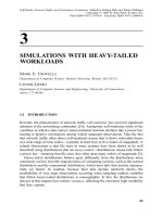
Fig. 1.4 Example of distinct counting problem

As previously mentioned, in many applications of aggregate query, we usually
need statistic information of road network such as vehicles counting (e.g., how many
vehicles have passed through Tiananmen Square from 8:00 to 9:00 this morning?).
As shown in Fig. 1.4, Q is the query area and there are some moving objects in it. At
time t1 , there are 5 objects in area Q. At time t1 +1, there are also 5 objects in area Q,
while some of these objects are the same as those at time t1 . At time t1 +2, there are
4 objects and some of these objects are still the same as those at times t1 and t1 +1.
If we want to know how many objects emerged from t1 to t1 +2 inside area Q, some
objects would be computed multiple times such as object1, object2, object3. This is
called distinct counting problem.
Aggregate query would gather massive information and process a large number
of moving objects. So it usually takes a lot of time. If we want to speed up query
process, it is better to reduce the number of counts. We require techniques which can
solve the distinct counting problem to improve the efficiency of aggregate query. In
the following chapters, we can use Sketch-based methods such as Sketch-RR tree
(to be mentioned in Sect. 4.3), DynSketch (to be mentioned in Sect. 4.4), MH (to be
mentioned in Sect. 4.5) methods to solve above problems in aggregate query.

1.5 Cloud for Intelligent Transportation

Cloud computing technology which has been developed in recent years is a new type
of computing patterns. Cloud computing embodies a new concept of information services. Cloud computing is the key technique of solving the problem of massive data
with its automated computer resource scheduling, deployment of high-speed information and excellent scalability. As an emerging computing and business model,
cloud computing is accelerating the processes of transportation information service
and information industry. Rapid development of cloud computing in the field of
intelligent transportation applications has positive significance to improve the integrated information processing capacity of the cities and promote the upgrading of
the industrial optimization and the structures. At the same time, cloud computing


1.5 Cloud for Intelligent Transportation

9

is promoting the transformation of the mode economic development, which has a
broad market prospect.
Intelligent transportation cloud is based on the data streams of the road networks.
Intelligent transportation cloud uses the excellent data processing capabilities of
cloud computing to improve the performance of the intelligent transportation systems
(ITS) as well as its scalability, reliability and cost benefits, and it provides strong
support for intelligent transportation system.

1.6 Summary
Intelligent Transportation System (ITS) is based on the increasing demands of the
transportation development. It integrates information, communications, computers
and other technologies, and applies them in the field of transportation to build an
integrated system of people, roads and vehicles by utilizing advanced data communication technologies. Roadways play the role as a carrier which is used to limit the
activities of people and vehicles. Technologies in road network contribute to establish
a large, full-functioning, realtime, accurate and efficient transportation management
system. With the development of ITS, researches on the road network will get a wide
range of industry and academic attention. This chapter briefly introduced the road

networks modeling, index and query for moving objects and some typical problems
in the applications of road networks.


Chapter 2

Index Techniques

The efficiency of data access and storage is a key factor that affects the quality of
data service, and it can be significantly improved by effective index mechanism. Data
index is a structure used to organize data records and describe the location information
of data in physical storage medium. Index techniques can help us access record set
through multiple ways and effectively support many kinds of queries. There are two
kinds of index method in traditional database system: the first one is tree (e.g., B+ -tree
or B-tree) based index, and the second is hash based index. Search engine often uses
inverted file as its index method. Spatial and temporal data indexes (e.g. R-tree and
its variants, K-D-tree and its variants, and space filling curves) are mainly extended
from traditional database index. This book centers on index and query techniques
in road network. As a complicated data structure, road network not only contains
static spatial data, such as roads, lakes, and buildings, but also includes dynamical
spatio-temporal data, e.g., the location information of mobile objects. So, to index
road network we must use various types of current index techniques holistically. In
order to analyze the index methods in road network well, in this chapter, we briefly
examine the typical indexes proposed in the literature and present a basic description
on them.

2.1 Binary-Tree Based Index Techniques
The binary search tree is a basic data structure for representing data items whose
index values are arranged in some linear order. The idea of repetitively partitioning
a data space has been adopted and generalized in many sophisticated indexes. In this

section, we will examine indexes originated from the basic structure and concept of
binary search trees.
Finally, we would like to further emphasize that solutions to all above mentioned
issues require close and efficient collaborations between the computer scientists
and the application developers. High performance index techniques can only be
developed with a through understanding of the usage of spatial data, including the
© Springer International Publishing Switzerland 2015
J. Feng and T. Watanabe, Index and Query Methods in Road Networks,
Smart Innovation, Systems and Technologies 29,
DOI 10.1007/978-3-319-10789-9_2

11


12

2 Index Techniques

access patterns and the post processing after data brought into memory. At the same
time, application developers may be able to provide certain services or tune their
algorithms to avoid some of the limitations of underlying indexing mechanism.

2.1.1 kd-Tree
A kd-tree [3] (short for multi-dimensinal binary search tree) is a space-partitioning
data structure for organizing points in a multi-dimensional space, which was introduced by Bentley in 1975. The kd-tree is a natural generalization of the well-known
binary search tree to handle the case of a single record having multiple keys. Differed
from the binary tree, a node in kd-tree (Fig. 2.1) is a k-dimensional point and serves
two purposes: representing an actual data point and giving the direction of a search.
In every level, there is a discriminator whose value is between 0 and k   1 inclusive,
which indicates the key on which the branching depends. A node P has two children,

a left son LOSON(P) and a right son HISON(P). If the discriminator value of node
P is the jth key (attribute), the jth key of any node in the HISON(P) is greater than
or equal to that of node P. This feature enables the range along each dimension to be

(a)

(b)

Fig. 2.1 Example of kd-tree. a Tree structure. b Planar structure


2.1 Binary-Tree Based Index Techniques

13

defined during a tree traversal such that the ranges are smaller in the lower levels of
the tree. To keep this property, deletion will probably cause successive replacements.
In order to reduce the cost of deletion, Bentley proposed a non-homogeneous kd-tree
in 1979 [4]. Unlike a homogeneous index, a non-homogeneous index does not store
data in the internal nodes and its internal nodes are used only as directories. The kdtree has been the subject of intensive research over the past decades. Many variants
have been proposed in the literature to improve the performance of the kd-tree with
respect to issues such as clustering, searching, storage efficiency and balancing.

2.1.2 K-D-B-Tree
To improve the paging capability of the kd-tree, Robinson proposed the K-D-B tree
[5] which combines the properties of kd-tree [3] and B-tree [6, 7].The K-D-B tree
consists of two basic parts: region pages (internal node) and point pages (leaf node)
(see Fig. 2.2). While point pages contain object identifiers, region pages store the
descriptions of subspaces in which the data points are stored and the pointers to
descendant pages. In K-D-B tree, these subspaces are explicitly stored in a region

page. These subspaces such as S11, S12, S13, are pairwise disjoint and together they
span the rectangular subspace of the current region page (e.g., S1), a subspace in the
parent region page.
When inserting a new point into a full point page, a split will happen. The point
page is split so that the two resultant point pages will contain almost the same number
of data points. Note that the spit of a point page requires an extra entry of a new point
page. This entry will be inserted into the parent region page. Therefore, the split of
a point page may cause the parent region page to split as well, which may further
ripple all the way to the root. Thus the tree is always perfectly height-balanced.

(b)
(a)

Fig. 2.2 Example of K-D-B tree. a Area devision. b Tree structure


14

2 Index Techniques

When a region page is split, the entries are partitioned into two groups such that
both have almost the same number of entries. A hyperplane is used to split the space of
a region page into two subspaces and this hyperplane may cut across the subspaces of
some entries. Consequently, the subspaces that intersect with the splitting hyperplane
must also be split so that the new subspaces are totally contained in the resultant
region pages. If the constraint of splitting a region page into two, containing the
same number of entries is not enforced, then downward propagation of split may be
avoided. The choice of the dimension for splitting and the splitting point would be
chosen so that both resultant pages have almost the same number of entries and the
number of splitting is minimized.

The upward propagation of a split would not cause the underflow of pages, but the
downward propagation is detrimental to storage efficiency because a page may contain less than the usual threshold, typically half of the page capacity. To avoid unacceptabe low storage utilization, local reorganization can be performed. For example,
two or more pages whose data space forms a rectangular space and they having the
same parent can be merged followed by a re-split if the resultant page overflows.

2.1.3 BSP-Tree
A Binary Space Partitioning tree (or BSP-tree) [8, 9] is a data structure that is used
to organize objects within a space. Like kd-trees, BSP-trees are binary trees that
represent a recursive subdivision of the universe into subspaces by means of (d   1)dimensional hyperplanes. Each subspace is subdivided independently according to
its history and other subspaces. The choice of the partitioning hyperplanes depends
on the distribution of the data objects in a given subspace. The decomposition usually
continues until the number of objects in each subspace is below a given threshold.
The resulting partition of the universe can be represented by a BSP-tree in which
each hyperplane corresponds to an interior node of the tree and each subspace corresponds to a leaf. Each leaf stores references to those objects that are contained in
the corresponding subspace.
Binary space partitioning was developed in the context of 3D computer graphics,
where the structure of a BSP-tree allows spatial information about the objects in
a scene that is useful in rendering, such as their ordering from front-to-back with
respect to a viewer at a given location, to be accessed rapidly. Other applications
include performing geometrical operations with shapes (constructive solid geometry)
in CAD, collision detection in robotics and 3D video games, ray tracing and other
computer applications that involve handling of complex spatial scenes.

2.1.4 Matsuyama’s kd-Tree
While most kd-trees are proposed as point access methods, the kd-tree proposed
by Matsuyama et al. [10] is designed for two-dimensional non-zero sized spatial


2.1 Binary-Tree Based Index Techniques

15

objects by supporting duplications of objects. The directory is a kd-tree, and for each
leaf node, a data page is associated. A data page contains the identifiers of objects
which are partially or totally included in its data space. Objects that overlap multiple
un-partitioned data space are duplicated in respective data pages.
Matsuyama’s kd-tree is searched like a conventional kd-tree. However, to insert
an object, the object identifier needs to be inserted into all the pages with subspaces
that intersect with the data object. It is quite common that object identifiers may be
duplicated in more than one page, particularly when the sizes of objects are large.
Whenever a page overflows, the page is split with a partition being introduced along
the longer side of the rectangle. The subspace is partitioned into two subspaces and
the two new pages contain all objects that intersect with their subspace.
To delete an object, it is necessary to search all leaf nodes with subspaces that
intersect with the data object and delete all identifiers referring to the data objects.
If the deletion of an object causes a page to be empty, the corresponding leaf node
should be marked NIL. To simplify the deletion algorithm, the underflowed data
pages do not need to be merged.
Matsuyama’s kd-tree is one of the earlier indexing structures adopting the object
duplication approach. Such an index is not suitable for indexing large objects as the
overhead of redundant storage can be very high.

2.1.5 4d-Tree
The kd-tree can be used to index two-dimensional rectangular objects by mapping
the objects into points in a 4-dimensional space. Each two-dimensional rectangular
described by (x1 , y1 ) and (x2 , y2 ), is treated as a four attribute tuple (x1 , x2 , y1 , y2 ).
The discriminator is used cyclically and the nodes at the same level use the same
discriminator. In [11], the issues involved in mapping the data structure onto pages
in secondary memory were not addressed. The same approach for the K-D-B tree
[5] was suggested by Banerjee and Kim [12]. The structure is known as the 4d-tree.

At each node of the 4d-tree, a discriminator (x1 , x2 , y1 , y2 ), discriminator value
and pointers to two child nodes are stored. A two-dimensional subspace is associated
with each node and as the tree is traversed during query, starting from the root, these
subspaces are successively pruned. Let the query region be (q x1 , q x2 , qy1 , qy2 ).
Then, at each internal node, one of the conditions, x1 q x2 , x2 q x1 , y1 qy2 or
y2 qy1 , has to be used depending on the discriminator stored in that node in order
to determine whether both subtrees or only one of the subtrees need to be searched.
The important part in the search algorithm is the determination of the subspaces
that bound the objects in the LO (le f t) and HI (right) subtrees. Traversal starts at the
root with the map as the associated space. Assume that the left discriminator is X 1 ,
the LO subtree contains objects whose X 1 coordinate is less than the discriminator
value, and the HI subtree contains objects whose X 1 coordinate is greater than the
discriminator value. The X 1 values of the HI subspace are bounded below by the
discriminator value and this fact can be used to reduce the subspace associated with