Macroeconomics pearson new international edition

Macroeconomics

Macroeconomics
Robert J. Gordon
Twelfth Edition

Gordon
Twelfth Edition

ISBN 978-1-29202-207-9

9 781292 022079

www.ebook3000.com


Macroeconomics
Robert J. Gordon
Twelfth Edition


Pearson Education Limited
Edinburgh Gate
Harlow
Essex CM20 2JE
England and Associated Companies throughout the world
Visit us on the World Wide Web at: www.pearsoned.co.uk
© Pearson Education Limited 2014
All rights reserved. No part of this publication may be reproduced, stored in a retrieval system, or transmitted
in any form or by any means, electronic, mechanical, photocopying, recording or otherwise, without either the
prior written permission of the publisher or a licence permitting restricted copying in the United Kingdom

issued by the Copyright Licensing Agency Ltd, Saffron House, 6–10 Kirby Street, London EC1N 8TS.
All trademarks used herein are the property of their respective owners. The use of any trademark
in this text does not vest in the author or publisher any trademark ownership rights in such
trademarks, nor does the use of such trademarks imply any affiliation with or endorsement of this
book by such owners.

ISBN 10: 1-292-02207-8
ISBN 13: 978-1-292-02207-9

British Library Cataloguing-in-Publication Data
A catalogue record for this book is available from the British Library
Printed in the United States of America

www.ebook3000.com


P

E

A

R

S

O

N

C U

S T O

M

L

I

B

R

A

R Y

Table of Contents

1. What Is Macroeconomics?
Robert J. Gordon

1

2. The Measurement of Income, Prices, and Unemployment
Robert J. Gordon

25

3. Income and Interest Rates: The Keynesian Cross Model and the IS Curve
Robert J. Gordon

57

4. Strong and Weak Policy Effects in the IS-LM Model
Robert J. Gordon

93

5. Financial Markets, Financial Regulation, and Economic Instability
Robert J. Gordon

129

6. The Government Budget, the Government Debt, and the Limitations of Fiscal Policy
Robert J. Gordon

167

7. International Trade, Exchanges Rates, and Macroeconomic Policy
Robert J. Gordon

201

8. Aggregate Demand, Aggregate Supply, and the Great Depression
Robert J. Gordon

243

9. Inflation: Its Causes and Cures
Robert J. Gordon

279

10. The Goals of Stabilization Policy: Low Inflation and Low Unemployment
Robert J. Gordon

329

11. the Theory of Economic Growth
Robert J. Gordon

375

12. The Big Questions of Economic Growth
Robert J. Gordon

407

13. The Goals, Tools, and Rules of Monetary Policy
Robert J. Gordon

445

I


14. The Economics of Consumption Behavior
Robert J. Gordon

479

15. The Economics of Investment Behavior
Robert J. Gordon

517

16. New Classical Macro and New Keynesian Macro
Robert J. Gordon

543

17. Conclusion: Where We Stand
Robert J. Gordon

573

Appendix: International Annual Time Series Data for Selected Countries: 1960-2010
Robert J. Gordon

599

Glossary
Robert J. Gordon

609

Index

617

II

www.ebook3000.com


What Is Macroeconomics?

Business will be better or worse.
—Calvin Coolidge, 1928

1 How Macroeconomics Affects
Our Everyday Lives
Macroeconomics is concerned with the big economic issues that determine your
own economic well-being as well as that of your family and everyone you know.
Each of these issues involves the overall economic performance of the nation
rather than whether one particular individual earns more or less than another.
The nation’s overall macroeconomic performance matters, not only for its
own sake but because many individuals experience its consequences. The
Global Economic Crisis that began in late 2007 has created enormous losses
of income and jobs for millions of American families. Not only were almost
15 million people unemployed in late 2010, but many more have given up
looking for jobs, have been forced to work part-time instead of full-time, or
have experienced pay cuts or furlough days when they have not been paid.
By one estimate, more than half of American families since 2007 have experienced the job loss of a family member, a pay cut, or being forced to work parttime instead of full-time.
Macroeconomic performance can also determine whether inflation will
erode the value of family savings, as occurred in the 1970s when the annual
inflation rate reached 10 percent. Today’s students also care about economic
growth, which will determine whether in their future lives they will have a

higher standard of living than their parents do today.

Macroeconomics is the study
of the major economic totals,
or aggregates.

The Global Economic Crisis
is the crisis that began in 2007
that simultaneously depressed
economic activity in most of the
world’s economies.

The “Big Three” Concepts of Macroeconomics
Each of these connections between the overall economy and the lives of individuals involves a central macroeconomic concept introduced in this chapter—
unemployment, inflation, and economic growth. The basic task of macroeconomics is to study the causes of good or bad performance of these three
concepts, why each matters to individuals, and what (if anything) the government can do to improve macroeconomic performance. While there are numerous other important macroeconomic concepts, we start by focusing just on
these, which are the “Big Three” concepts of macroeconomics:
1. The unemployment rate. The higher the overall unemployment rate, the
harder it is for each individual who wants a job to find work. College seniors who want permanent jobs after graduation are likely to have fewer job
offers if the national unemployment rate is high, as in 2009–10, than low, as

The unemployment rate
is the number of persons
unemployed (jobless individuals
who are actively looking for work
or are on temporary layoff)
divided by the total of those
employed and unemployed.

From Chapter 1 of Macroeconomics, Twelfth Edition. Robert J. Gordon. Copyright © 2012 by Pearson Education, Inc.

Published by Pearson Addison Wesley. All rights reserved.

1


What Is Macroeconomics?

The inflation rate is the
percentage rate of increase in
the economy’s average level
of prices.

Productivity is the aggregate
output produced per hour.

in 2005–2007. All adults fear a high unemployment rate, which raises the
chances that they will be laid off, be unable to pay their bills, have their
cars repossessed, lose their health insurance, or even lose their homes
through mortgage foreclosures. In “bad times,” when the unemployment
rate is high, crime, mental illness, and suicide also increase. The widespread consensus that unemployment is the most important macroeconomic issue has been further highlighted by the dismal labor market of
2009–10, when fully half of the unemployed were jobless for more than
six months. And the recognized harm created by high unemployment is
nothing new. Robert Burton, an English clergyman, wrote in 1621 that
“employment is so essential to human happiness that indolence is justly
considered the mother of misery.”
2. The inflation rate. A high inflation rate means that prices, on average, are
rising rapidly, while a low inflation rate means that prices, on average, are
rising slowly. An inflation rate of zero means that prices remain essentially
the same, month after month. In inflationary periods, retired people, or
those about to retire, lose the most, since their hard-earned savings buy less

as prices go up. Even college students lose as the rising prices of room,
board, and textbooks erode what they have saved from previous summer
and after-school jobs. While a high inflation rate harms those who have
saved, it helps those who have borrowed. Great harm comes from this
capricious aspect of inflation, taking from some and giving to others.
People want their lives to be predictable, but inflation throws a monkey
wrench into individual decision making, creating pervasive uncertainty.
3. Productivity growth. “Productivity” is the aggregate output per hour of
work that a nation produces in total goods and services; it was about $61
per worker-hour in the United States in 2010. The faster aggregate productivity grows, the easier it is for each member of society to improve his or
her standard of living. If productivity were to grow at 3 percent from 2010
to the year 2030, U.S. productivity would rise from $61 per worker-hour to
$111 per worker-hour. When multiplied by all the hours worked by all the
employees in the country, this extra $50 per worker-hour would make it
possible for the nation to have more houses, cars, hospitals, roads, schools,
and to combat greenhouse gas emissions that worsen global warming.
But if the growth rate of productivity were zero instead of 3 percent,
U.S. productivity would remain at $61 in the year 2030. To have more
houses and cars, we would have to sacrifice by building fewer hospitals
and schools. Such an economy, with no productivity growth, has been
called the “zero-sum society,” because any extra good or service enjoyed
by one person requires that something be taken away from someone else.
Many have argued that the achievement of rapid productivity growth and
the avoidance of a zero-sum society form the most important macroeconomic challenge of all.
The first two of the “Big Three” macroeconomic concepts, the unemployment and inflation rates, appear in the newspaper every day. When economic
conditions are poor—as in 2009–10—daily headlines announce that one large
company or another is laying off thousands of workers. In the past, sharp
increases in the rate of inflation have also made headlines, as when the price of
gasoline jumped during 2006–08. The third major concept, productivity growth,
has received widespread attention since 1995 as a source of an improving

American standard of living compared to that in Europe and Japan.

2

www.ebook3000.com


What Is Macroeconomics?

Macroeconomic concepts also play a big role in politics. Incumbent political
parties benefit when unemployment and inflation are relatively low, as in
the landslide victories of Lyndon Johnson in 1964 and Richard Nixon in 1972.
Incumbent presidents who fail to gain reelection often are the victims of a sour
economy, as in the cases of Herbert Hoover in 1932, Jimmy Carter in 1980, and
more recently George W. Bush in 2008. The defeat of Al Gore by George W. Bush
in 2000 was an exception since the strong economy of 2000 should have helped
Gore’s incumbent Democratic party win the presidency.

GLOBAL ECONOMIC CRISIS FOCUS
What Makes It Unique?
The Global Economic Crisis that started in 2008 is by most measures the most
severe downturn since the Great Depression of the 1930s. Its severity is most
apparent in the high level of the unemployment rate (10 percent) reached in
2009–10, in the relatively long duration of unemployment suffered by those
who lost their jobs, and in the prediction that the unemployment rate would
not return to its normal level of around 5 percent until perhaps 2015 or 2016.
Thus, of our three big macro concepts, the Global Economic Crisis mainly affected the unemployment rate, while the inflation rate remained low and productivity growth was relatively robust.

2

Defining Macroeconomics

How Macroeconomics Differs from Microeconomics
Most topics in economics can be placed in one of two categories: macroeconomics or microeconomics. Macro comes from a Greek word meaning large; micro
comes from a Greek word meaning small. Put another way, macroeconomics
deals with the totals, or aggregates, of the economy, and microeconomics deals
with the parts.
Microeconomics is devoted to the relationships among the different parts of
the economy. For example, in micro we try to explain the wage or salary of one
type of worker in relation to another. For example, why is a professor’s salary
more than that of a secretary but less than that of an investment banker? In contrast, macroeconomics asks why the total income of all citizens rises strongly in
some periods but declines in others.

An aggregate is the total
amount of an economic
magnitude for the economy
as a whole.

Economic Theory: A Process of Simplification
Economic theory helps us understand the economy by simplifying complexity.
Theory throws a spotlight on just a few key relations. Macroeconomic theory
examines the behavior of aggregates such as the unemployment rate and the
inflation rate while ignoring differences among individual households. It studies the causes and possible cures of the Global Economic Crisis at the level of
individual nations, instead of trying to explain why some individuals are more
prone than others to losing their jobs.
It is this process of simplification that makes the study of economics so
exciting. By learning a few basic macroeconomic relations, you can quickly

3

What Is Macroeconomics?

learn how to sift out the hundreds of irrelevant details in the news in order to
focus on the few key items that foretell where the economy is going. You also
will begin to understand which national and personal economic goals can be
attained and which are “pie in the sky.” You will learn when it is fair to credit
a president for strong economic performance or blame a president for poor
performance.

3

Gross domestic product is
the value of all currently
produced goods and services
sold on the market during a
particular time interval.

Actual real GDP is the value
of total output corrected for
any changes in prices.

Natural real GDP designates
the level of real GDP at which
the inflation rate is constant,
with no tendency to accelerate
or decelerate.

Actual and Natural Real GDP

We have learned that the “Big Three” macroeconomic concepts are the unemployment rate, the inflation rate, and the rate of productivity growth. Linked to
each of these is the total level of output produced in the economy. The higher
the level of output, the lower the unemployment rate. The higher the level of
output, the faster tends to be the rate of inflation. Finally, for any given number
of hours worked, a higher level of output automatically boosts output per
hour, that is, productivity.
The official measure of the economy’s total output is called gross domestic
product and is abbreviated GDP. Real GDP includes all currently produced
goods and services sold on the market within a given time period and excludes
certain other types of economic activity. As you will also learn, the adjective
“real” means that our measure of output reflects the quantity produced, corrected for any changes in prices.
Actual real GDP is the amount an economy actually produces at any
given time. But we need some criterion to judge the desirability of that level
of actual real GDP. Perhaps actual real GDP is too low, causing high unemployment. Perhaps actual real GDP is too high, putting upward pressure on
the inflation rate. Which level of real GDP is desirable, neither too low nor
too high? This intermediate compromise level of real GDP is called “natural,”
a level of real GDP in which there is no tendency for the rate of inflation to
rise or fall.
Figure 1 illustrates the relationship between actual real GDP, natural real
GDP, and the rate of inflation. In the upper frame the red line is actual real
GDP. The lower frame shows the inflation rate. The thin dashed vertical lines
connect the two frames. The first dashed vertical line marks time period t0.
Notice in the bottom frame that the inflation rate is constant at t0, neither
speeding up nor slowing down.
By definition, natural real GDP is equal to actual real GDP when the inflation rate is constant. Thus, in the upper frame, at t0 the red actual real GDP line
is crossed by the black natural real GDP line. To the right of t0, actual real GDP
falls below natural real GDP, and we see in the bottom frame that inflation
slows down. This continues until time period t1, when actual real GDP once
again is equal to natural real GDP. Here the inflation rate stops falling and is
constant for a moment before it begins to rise.

This cycle repeats itself again and again. Only when actual real GDP is equal
to natural real GDP is the inflation rate constant. For this reason, natural real GDP
is a compromise level to be singled out for special attention. During a period of
low actual real GDP, designated by the blue area, the inflation rate slows down.
During a period of high actual real GDP, designated by the shaded red area, the
inflation rate speeds up.

4

www.ebook3000.com


What Is Macroeconomics?

Why Too Much Real GDP Is Undesirable

Natural
real GDP

Real GDP

Actual
real GDP

Figure 1 The Relation Between
Actual and Natural Real GDP and
the Inflation Rate
In the upper frame the solid black line
shows the steady growth of natural real
GDP—the amount the economy can

produce at a constant inflation rate. The
red line shows the path of actual real
GDP. In the blue region in the top frame,
actual real GDP is below natural real
GDP, so the inflation rate, shown in the
bottom frame, slows down. In the region
designated by the red area, actual real
GDP is above natural real GDP, so in the
bottom frame inflation speeds up.

Inflation rate

Inflation
rate

Inflation
slows
down
t0

Inflation
speeds
up
t1

Inflation
speeds
up
t2

t3

Inflation
slows
down
t4

Time

Unemployment: Actual and Natural
When actual real GDP is low, many people lose their jobs, and the unemployment rate is high, as shown in Figure 2. The top frame duplicates Figure 1
exactly, comparing actual real GDP with natural real GDP. The blue line in the
bottom frame is the actual percentage unemployment rate, the first of the three
central concepts of macroeconomics. The thin vertical dashed lines connecting
the upper frame and lower frame show that whenever actual and natural real
GDP are equal in the top frame, the actual unemployment rate is equal to the
natural rate of unemployment in the bottom frame.
The definition of the natural rate of unemployment corresponds exactly to
natural real GDP, describing a situation in which there is no tendency for the inflation rate to change. When the actual unemployment rate is high, actual real
GDP is low (shown by blue shading in both frames), and the inflation rate
slows down. In periods when actual real GDP is high and the economy prospers, the actual unemployment rate is low (shown by red shading in both
frames) and the inflation rate speeds up. It is easy to remember the mirrorimage behavior of real GDP and the unemployment rate. We use the shorthand

The natural rate of
unemployment designates the
level of unemployment at which
the inflation rate is constant,
with no tendency to accelerate
or decelerate.

5


What Is Macroeconomics?

Unemployment Cycles Are
the Mirror Image of Real GDP Cycles

Natural
real GDP

Real GDP

Actual
real GDP

Unemployment rate (percent)

Figure 2 The Behavior Over Time
of Actual and Natural Real GDP and
the Actual and Natural Rates of
Unemployment
When actual real GDP falls below natural
real GDP, designated by the blue shaded
areas in the top frame, the actual
unemployment rate rises above the
natural rate of unemployment as
indicated in the bottom frame. The red
shaded areas designate the opposite
situation. When we compare the blue

shaded areas of Figures 1 and 2,
we see that the time intervals when
unemployment is high (1–2) also
represent time intervals when inflation
is slowing down (1–1). Similarly, the red
shaded areas represent time intervals
when inflation is speeding up and
unemployment is low.

Actual
unemployment
rate

Natural
unemployment rate

t0

t1

t2

t3

t4

Time

The GDP gap is the percentage
difference between actual real

GDP and natural real GDP.
Another name for this concept
is the “output gap.”
The unemployment gap is
the difference between the
actual unemployment rate
and the natural rate of
unemployment.

label GDP gap for the percentage difference between actual real GDP and natural real GDP. We use the parallel shorthand label unemployment gap for the
difference between the actual unemployment rate and the natural rate of unemployment. In recessions when the GDP gap is negative, the unemployment gap
is positive, and both of the gaps are represented by the blue shaded areas in
Figure 2. In highly prosperous periods like the late 1990s, the GDP gap is
positive and the unemployment gap is negative, as indicated by the red shaded
areas in Figure 2. Another name for the GDP gap is the “output gap.”
Figures 1 and 2 summarize a basic dilemma faced by government policymakers who are attempting to achieve a low unemployment rate and a low
inflation rate at the same time. If the inflation rate is high, lowering it requires a
decline in actual real GDP and an increase in the actual unemployment rate.
This happened in the early 1980s, when inflation was so high that the government deliberately pushed unemployment to its highest level since the 1930s. If,
to the contrary, the policymaker attempts to provide jobs for everyone and
keep the actual unemployment rate low then the inflation rate will speed up, as
occurred in the 1960s and late 1980s.

6

www.ebook3000.com


What Is Macroeconomics?

Real GDP and the Three Macro Concepts
The total amount that the economy produces, actual real GDP, is closely related
to the three central macroeconomic concepts introduced earlier in this chapter.
First, as we see in Figure 2, the difference between actual and natural real GDP
moves inversely with the difference between the actual and natural unemployment rates. When actual real GDP is high, unemployment is low, and vice versa.
The second link is with inflation, since inflation tends to speed up when
actual real GDP is higher than natural real GDP (as in Figure 1). The third
link is with productivity, which is defined as actual real GDP per hour; data on
actual real GDP are required to calculate productivity.
Each of these links with the central macroeconomic concepts requires that
actual real GDP be compared with something else in order to be meaningful. It
must be compared to natural real GDP to provide a link with unemployment
and inflation, or it must be divided by the number of hours worked to compute
productivity. Actual real GDP by itself, without any such comparison, is not
meaningful, which is why it is not included on the list of the three major macro
concepts.

SELF-TEST 1
1. When actual real GDP is above natural real GDP, is the actual unemployment
rate above, below, or equal to the natural unemployment rate?
2. When actual real GDP is below natural real GDP, is the actual unemployment
rate above, below, or equal to the natural unemployment rate?
3. When the actual unemployment rate is equal to the natural rate of unemployment, is the actual rate of inflation equal to the natural rate of inflation?

4 Macroeconomics in the
Short Run and Long Run
Macroeconomic theories and debates can be divided into two main groups:
(1) those that concern the “short-run” stability of the economy, and (2) those
that concern its “long-run” growth rate. Much of macroeconomic analysis concerns the first group of topics involving the short run, usually defined as a period lasting from one year to five years, and focuses on the first two major
macroeconomic concepts introduced in Section 1, the unemployment rate

and the inflation rate. We ask why the unemployment rate and the inflation
rate over periods of a few years are sometimes high and sometimes low, rather
than always low as we would wish. These ups and downs are usually called
“economic fluctuations” or business cycles. Much of this text concerns the
causes of these cycles and the efficacy of alternative government policies to
dampen or eliminate the cycles.
The other main topic in macroeconomics concerns the long run, which is a
longer period ranging from one decade to several decades. It attempts to
explain the rate of productivity growth, the third key concept introduced in
Section 1, or more generally, economic growth. Learning the causes of growth
helps us predict whether successive generations of Americans will be better off
than their predecessors, and why some countries remain so poor in a world

Business cycles consist of
expansions occurring at about
the same time in many economic
activities, followed by similarly
general recessions and recoveries.
Economic growth is the topic
area of macroeconomics that
studies the causes of sustained
growth in real GDP over periods
of a decade or more.

7


What Is Macroeconomics?

where other countries by contrast are so rich. The remarkable achievement of

China in achieving economic growth of 8 to 9 percent per year consistently over
the past three decades raises a new question about economic growth—how long
will it take the Chinese economy to catch up to the American level of real GDP
per person?

The Short Run: Business Cycles
The main short-run concern of macroeconomists is to minimize fluctuations in
the unemployment and inflation rates. This requires that fluctuations in real
GDP be minimized.
Figure 3 contrasts two imaginary economies: “Volatilia” in the left frame
and “Stabilia” in the right frame. The black “natural real GDP” lines in both
frames are absolutely identical. The two economies differ only in the size of their
business cycles, shown by the size of their GDP gap, which is simply the difference between actual and natural real GDP shown by blue and red shading.
In the left frame, Volatilia is a macroeconomic hell, with severe business cycles and large gaps between actual and natural real GDP. In the right frame,
Stabilia is macroeconomic heaven, with mild business cycles and small gaps
between actual and natural real GDP. All macroeconomists prefer the economy
depicted by the right-hand frame to that depicted by the left-hand frame. But
the debate between macro schools of thought starts in earnest when we ask
how to achieve the economy of the right-hand frame. Active do-something
policies? Do-nothing, hands-off policies? There are economists who support
each of these alternatives, and more besides. But everyone agrees that Stabilia

Natural real GDP

Natural real GDP

Real GDP

Real GDP

Economic Failure and Success

Actual real GDP

Actual real GDP

Time
(a) Volatilia

Time
(b) Stabilia

Figure 3 Business Cycles in Volatilia and Stabilia
The left frame shows the huge business cycles in a hypothetical nation called Volatilia.
Short-run macroeconomics tries to dampen business cycles so that the path of actual
real GDP is as close as possible to natural real GDP, as shown in the right frame for a
nation called Stabilia.

8

www.ebook3000.com


What Is Macroeconomics?

A Succession of Cycles

Peak Trough
Real
output

Expansion

Expansion

Recession

Recession

Peak Trough

Recession

Real GDP

Peak Trough

Figure 4 Basic Business-Cycle Concepts
The real output line exhibits a typical
succession of business cycles. The highest
point reached by real output in each cycle
is called the peak and the lowest point the
trough. The recession is the period between
peak and trough; the expansion is the period
between the trough and the next peak.

Time

is a more successful economy than Volatilia. To achieve the success of Stabilia,
Volatilia must find a way to eliminate its large real GDP gap.

The hallmark of business cycles is their pervasive character, which affects
many different types of economic activity at the same time. This means that
they occur again and again but not always at regular intervals, nor are they the
same length. Business cycles in the past have ranged in length from one to
twelve years.1 Figure 4 illustrates two successive business cycles in real output. Although a simplification, Figure 4 contains two realistic elements that
have been common to most real-world business cycles. First, the expansions
last longer than the recessions. Second, the two business cycles illustrated in
the figure differ in length.

The Long Run: Economic Growth
For a society to achieve an increasing standard of living, total output per person
must grow, and such economic growth is the long-run concern of macroeconomists. Look at Figure 5, which contrasts two economies. Each has mild business cycles, like Stabilia in Figure 3. But in Figure 5, the left frame presents a
country called “Stag-Nation,” which experiences very slow growth in real GDP.
In contrast, the right-hand frame depicts “Speed-Nation,” a country with very
fast growth in real GDP. If we assume that population growth in each country is
the same, then growth in output per person is faster in Speed-Nation. In SpeedNation everyone can purchase more consumer goods, and there is plenty of output left to provide better schools, parks, hospitals, and other public services. In
Stag-Nation people must constantly face debates, since more money for schools
or parks requires that people sacrifice consumer goods.

1

A comprehensive source for the chronology of and data on historical business cycles, as well as
research papers by distinguished economists, is Robert J. Gordon, ed., The American Business Cycle:
Continuity and Change (Chicago: University of Chicago Press, 1986). An up-to-date chronology and
a discussion of the 2007–09 recession can be found at www.nber.org/cycles/cyclesmain.html.

9


What Is Macroeconomics?

Economic Failure and Success in Another Dimension

Real GDP

Real GDP

Natural real GDP

Natural real GDP

Actual real GDP

Actual real GDP

Time

Time
(b) Speed-Nation

(a) Stag-Nation

Figure 5 Economic Growth in Stag-Nation and Speed-Nation
In both frames the business cycle has been tamed, but in the left frame there is almost no
economic growth, while economic growth in the right frame is rapid. For Speed-Nation
there can be more of everything, while Stag-Nation in the left frame is a “zero-sum
society,” in which an increase in one type of economic activity requires that another
economic activity be cut back.

Over the past decade, countries like Stag-Nation include Germany, Italy,

and Japan. Countries like Speed-Nation include China and India. The United
States has been between these extremes.
How do we achieve faster economic growth in output per person?
We study the sources of economic growth and the role of government policy in
helping to determine the growth in America’s future standard of living, as well
as the reasons why some countries remain so poor.

SELF-TEST 2
Indicate whether each item in the following list is more closely related to shortrun (business cycle) macro or to long-run (economic growth) macro:
1. The Federal Reserve reduces interest rates in a recession in an attempt to
reduce the unemployment rate.
2. The federal government introduces national standards for high school students in an attempt to raise math and science test scores.
3. Consumers cut back spending because news of layoffs makes them fear for
their jobs.
4. The federal government gives states and localities more money to repair
roads, bridges, and schools.

10

www.ebook3000.com


What Is Macroeconomics?

5 CASE STUDY

How Does the Global Economic Crisis
Compare to Previous Business Cycles?
This section examines U.S. macroeconomic history since the early twentieth
century. You will see that unemployment in the past four decades did not come

close to the extreme crisis levels of the 1930s.

Real GDP
Figure 6 is arranged just like Figure 2. But whereas Figure 2 shows hypothetical relationships, Figure 6 shows the actual historical record. In the top frame the
solid black line is natural real GDP, an estimate of the amount the economy could
have produced each year without causing acceleration or deceleration of inflation.
The red line in the top frame plots actual real GDP, the total production of
goods and services each year measured in the constant prices of 2005. Can you
pick out those years when actual and natural real GDP are roughly equal?
Some of these years were 1900, 1910, 1924, 1964, 1987, 1997, and 2007.
In years marked by blue shading, actual real GDP fell below natural real
GDP. A maximum deficiency occurred in 1933, when actual real GDP was only
64 percent of natural GDP; about 35 percent of natural real GDP was thus
“wasted,” that is, not produced. In some years actual real GDP exceeded natural
real GDP, shown by the shaded red areas. The largest red area occurred during
World War II in 1942–45.

Unemployment
In the middle frame of Figure 6, the blue line plots the actual unemployment
rate. By far the most extreme episode was the Great Depression, when the
actual unemployment rate remained above 10 percent for ten straight years,
1931–40. The black line in the middle frame of Figure 6 displays the natural
rate of unemployment, the minimum attainable level of unemployment that is
compatible with avoiding an acceleration of inflation. The red shaded areas
mark years when actual unemployment fell below the natural rate, and the
blue shaded areas mark years when unemployment exceeded the natural rate.
Notice now the relationship between the top and middle frames of Figure 6.
The blue shaded areas in both frames designate periods of low production, low
real GDP, and high unemployment, such as the Great Depression of the 1930s.
The red shaded areas in both frames designate periods of high production and

high actual real GDP, and low unemployment, such as World War II and other
wartime periods. ◆

GLOBAL ECONOMIC CRISIS FOCUS
How It Differs from 1982–83
The bottom frame of Figure 6 magnifies the middle frame by starting the plot in
1970 instead of 1900. Over the past four decades there have been three big recessions with unemployment reaching its peak in 1975, then 1982–83, and most
recently in 2009–10. The recent episode of high unemployment is more serious
(continued)

11


A Historical Report Card on Real GDP and Unemployment

15,000

Billions of 2005 dollars

10,000

Natural real GDP

1,000

300
1900

Actual real GDP

1910

1920

1930

1940

1950

1960

1970

1980

1990

2000

2010

1970

1980

1990

2000

2010

30
25

Actual unemployment rate

Percent

20
15
Natural unemployment rate
10
5
0
1900

1910

1920

1930

1940

1950

1960

10

Actual unemployment rate

9
8

Percent

7
6
5
4

Natural unemployment rate

3
2
1
0
1970

1980

1990

2000

2010

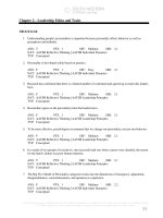
Figure 6 Actual and Natural GDP and Unemployment, 1900–2010
A historical report card for two important economic magnitudes. In the top frame the

black line indicates natural real GDP. The red line shows actual real GDP, which was
well below natural real GDP during the Great Depression of the 1930s and well above
it during World War II. In the middle frame the black line indicates the natural rate
of unemployment, and the blue line indicates the actual unemployment rate. Actual
unemployment was much higher during the Great Depression of the 1930s than at any
other time during the century. The bottom frame magnifies the middle frame to focus on
unemployment since 1970. There we see that the 2009–10 levels of high unemployment
were equivalent to 1982–83. However, the increase in unemployment was greater in
2007–10 than in 1980–82 since that economy started from a lower unemployment rate.

12

www.ebook3000.com


What Is Macroeconomics?

and harmful than in 1982–83 for several reasons. Notice that the unemployment
rate dropped sharply from 1983 to 1984, while the decline in the unemployment
rate in 2011–12 is forecast to be very slow. In the recent episode a larger share of
the unemployed have been without jobs for six months or more, and a much
larger share of the labor force than in 1982–83 has been forced to work on a parttime basis rather than their desired full-time status.

6

Macroeconomics at the Extremes

Most of macroeconomics treats relatively normal events. Business cycles occur,
and unemployment goes up and down, as does inflation. Economic growth
registers faster rates in some decades than in others. Yet there are times when

the economy’s behavior is anything but normal. The normal mechanisms of
macroeconomics break down, and the consequences can be dire. Three examples of unusual macroeconomic behavior involving our “Big Three” concepts
are the Great Depression of the 1930s, the German hyperinflation of the 1920s,
and the stark difference in economic growth between two Asian nations over
the past 50 years.

Unemployment in the Great Depression, 1929–40
The first of our “Big Three” macroeconomic concepts is the unemployment rate.
The most extreme event involving unemployment in recorded history was the
Great Depression of the 1930s. As is clearly visible in Figure 6 in the previous
section, real GDP collapsed between 1929 and 1933, and the unemployment rate
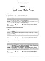
soared. A closer look at the decade of the 1930s is provided in Figure 7. For
contrast with the 1930s, the blue line displays the unemployment rate from 1998
to 2010. The unemployment rate during the Great Depression behaved quite
differently, as shown by the purple line, soaring from 3.2 percent in 1929 to
25.2 percent in 1933, and never falling below 10 percent until 1941. By 2010 the
unemployment rate had reached 9.5 percent, almost as high as it was in 1941.
In the United States, the Great Depression caused many millions of jobs to
disappear. College seniors could not find jobs. Stories of job hunting were unbelievable but true. For example, men waited all night outside Detroit employment
offices so they would be first in line the next morning. An Arkansas man walked
900 miles looking for work. So discouraged were Americans of finding jobs that
for the first (and last) time in American history, there were more emigrants than
immigrants. In fact, there were 350 applications per day from Americans who
wanted to settle in Russia. Since there was no unemployment insurance, how did
people live when there were no jobs? Wedding rings were sold, furniture pawned,
life insurance borrowed against, and money begged from relatives. Millions with
no resources moved aimlessly from city to city, sometimes riding on freight cars;
some cities tried to keep the wanderers out with barricades and shotguns.2
The Great Depression affected most of the industrialized world but was
most serious in the United States and in Germany. The Great Depression in

Germany led directly to Hitler’s takeover of power in 1933 and indirectly

2

Details in this paragraph are from William Manchester, The Glory and the Dream: A Narrative
History of America, 1932–72 (Boston: Little-Brown, 1973), pp. 33–35.

13


What Is Macroeconomics?

Unemployment in the 1930s Dwarfed Unemployment Since 1998

30

25

Unemployment rate (percent)

Unemployment rate, 1929–1941

20

15

10
Unemployment rate, 1998–2010
5

0
1929
1998

1931
2000

1933
2002

1935
2004

1937
2006

1939
2008

1941
2010

Figure 7 The Unemployment Rate from 1929–41 Compared with 1998–2010
The blue line displays the unemployment rate from 1998 to 2010, when the
unemployment rate ranged from 4 percent in 2000 to 10 percent in 2010. In contrast
the purple line exhibits the unemployment rate during the Great Depression; this
never fell below 14 percent the ten years from 1931 to 1940.
Source: Bureau of Labor Statistics.

caused the 50 million deaths of World War II. What caused the disastrous depression and what could have been done to avoid it? We need to study basic

macroeconomics first, and then we will examine the causes of the Great
Depression.

The German Hyperinflation of 1922–23
A hyperinflation can be defined as an inflation raging at a rate of 50 percent or more
per month. If a Big Mac cost $2 in January, a 50 percent monthly inflation would
raise the price to $3 in February, $4.50 in March, $6.75 in April, and onward until it
reached $173 in December! There were several examples of hyperinflation in the
twentieth century, most of them involving the experience of European countries
after World Wars I and II. The best known is the German hyperinflation, which
proceeded at 322 percent per month between August 1922 and November 1923; in
its final climactic days in October 1923, the inflation rate was 32,000 percent per
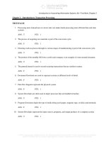
month! Figure 8 displays the German price level from 1920 to 1923. The price

14

www.ebook3000.com


What Is Macroeconomics?

When Sausages Cost 100 Billion Marks

1,000,000,000,000

Price level (in German marks)

1,000,000,000

1,000,000

1,000

1
1920

1921

1922

1923

1924

Figure 8 The German Price Level, 1920–23
The orange line shows the German price level, which increased from a little above 1 in
1920 and 1921 to 550 at the end of 1922 and to 100,000,000,000 in November 1923.

level goes from slightly above 1.0 in 1920 and early 1921 to 550 by the end of 1922
and about 100,000,000,000 at the end of 1923.
The basic cause of the German hyperinflation was the Versailles Peace Treaty,
which ended World War I and required payment of massive reparations by
Germany to Britain and France. The Germans were unwilling to obtain funds to
pay the reparations by raising taxes, so instead they ran huge government budget
deficits financed by printing paper money. When people realized the implications
of these deficits, they became less willing to hold money; it was both the rapid increase in the supply of money and the ever-declining demand for money that
combined to fuel the hyperinflation.3
The inflation decimated the savings of ordinary Germans. A farmer who
sold a piece of land for 80,000 marks as a nest egg for his old age could barely
buy a sandwich with the money a few years later. Elderly Germans can still

recall the days in 1923 when:
People were bringing money to the bank in cardboard boxes and laundry baskets.
As we no longer could count it, we put the money on scales and weighed it. I can
still see my brothers coming home Saturdays with heaps of paper money. When the
3

Data from Philip Cagan, “The Monetary Dynamics of Hyperinflation,” in Milton Friedman, ed.,
Studies in the Quantity Theory of Money (Chicago: University of Chicago Press, 1956), Table 1, p. 26.

15


What Is Macroeconomics?

shops reopened after the weekend they got no more than a breakfast roll for it.
Many got drunk on their pay because it was worthless on Monday.4

Just as the Great Depression helped to create resentments about the existing
government that turned voters to Hitler’s Nazi party, so bitter memories of lost
savings in the hyperinflation ten years earlier added to Hitler’s growing support. Very rapid inflation is not an ancient artifact lacking relevance for today.
Throughout the 1980s and 1990s several Latin American countries suffered from inflation rates of 1,000 percent per year or more. Recently, a devastating inflation broke out in the southern African nation of Zimbabwe, where
the inflation rate in October 2008 reached 210 billion percent per year!
Because the government failed to raise the wages of teachers and hospital
workers by even remotely the percentage by which prices had gone up, the
nation in 2007–09 was in a state of collapse, with schools and hospitals closing down. So severe was the hyperinflation that in early 2009 the government
cut 12 zeros off all types of currency and all prices, so that people would
trade in a banknote marked 1,000,000,000,000 and receive a new banknote
marked 1. In this chaotic environment more and more citizens turned to
using currencies of other countries, particularly the South African Rand.

Fast and Slow Growth in Asia
Neither the Great Depression nor the German hyperinflation had any significant effect on the American or German standard of living a decade or two later.
For effects that really matter over the decades, we need to look at the third of
our “Big Three” macroeconomic concepts: productivity growth. Differences in
growth rates that may appear small can compound over the decades and create
enormous differences in the standard of living of any economic unit, from individuals to nations. A classic example of the importance of rapid growth is illustrated in Figure 9, which displays real GDP per capita in South Korea and the
Philippines over the period 1960 to 2010.
In 1960, real GDP per capita in the Philippines was actually 20 percent
higher than in South Korea. But between 1960 and 2010, real GDP per capita
grew at 5.6 percent per year in South Korea compared to only 1.4 percent in the
Philippines. Figure 9 shows the wide gap that opened up between the
Korean and Philippine standards of living, with 2010 values of only $4,357
for the Philippines and $30,175 for South Korea. As a result of its superior
economic growth record, the average Korean in 2010 could save or consume
almost seven times as much as the average citizen of the Philippines. Stated another way, the Korean could consume everything enjoyed by the Philippine
citizen and then have almost six times as much left over. This extra output in
Korea is shown by the orange shading in Figure 9.
The outstanding achievement of South Korea has been duplicated in several other countries in East Asia, notably Hong Kong, Singapore, and Taiwan,
and more recently by China. What secrets have the Koreans learned about economic growth that the Philippine government and population have not
learned?

4

Alice Siegert, “When Inflation Ruined Germany,” Chicago Tribune, November 30, 1974.

16

www.ebook3000.com

What Is Macroeconomics?

South Korea Leaves the Philippines in the Dust

35,000

Real GDP per capita (2010 U.S. dollars)

30,000

25,000

20,000
South Korea
15,000

10,000

5,000

0
1960

Philippines

1965

1970

1975

1980

1985

1990

1995

2000

2005

2010

Figure 9 Per-Capita Real GDP, South Korea and the Philippines, 1960–2010
in 2010 U.S. Dollars
Per-capita real GDP in the Philippines barely grew from 1960 to 2008; the growth rate
between those years was only 1.4 percent per annum. In contrast, the growth rate in
Korea was 5.6 percent, enough to boost per-capita real GDP to a level fully 16 times
the 1960 value.
Source: Groningen Growth and Development Center.

7

Taming Business Cycles: Stabilization Policy

Macroeconomic analysts have two tasks: to analyze the causes of changes in important aggregates and to predict the consequences of alternative policy changes. In
policy discussions the group of aggregates that society cares most about—inflation,
unemployment, and the long-term growth rate of productivity—are called goals,

or target variables. When the target variables deviate from desired values, alternative policy instruments can be used in an attempt to achieve needed changes.
Instruments fall into three broad categories: monetary policies, which include control of the money supply and interest rates; fiscal policies, which include changes
in government expenditures and tax rates; and a third, miscellaneous group, which
includes policies to equip workers with skills they need to qualify for jobs.
How are target variables and policy instruments related to the three central
macroeconomic concepts introduced at the beginning of this chapter? All three

Target variables are aggregates
whose values society cares about.
Policy instruments are
elements that government
policymakers can manipulate
directly to influence target
variables.
Monetary policy tries to
influence target variables by
changing the money supply or
interest rate or both.
Fiscal policy tries to influence
target variables by manipulating
government expenditures and
tax rates.

17


What Is Macroeconomics?

INTERNATIONAL PERSPECTIVE
Differences Between the United States and Europe

Before and During the Global Economic Crisis

O

ne result of the internationalization of macroeconomics is the increased attention to the relative economic performance of major countries
or regions in the world, such as the United States versus
Europe or Asia. We learn from these comparisons that
performance differs over time. Compared to Europe,
the United States did not perform well from 1960 to
1985 but then started to improve and performed much
better than Europe after 1995, at least until the 2007 start
of the Global Economic Crisis.
Good performance means the achievement of low
unemployment, low inflation, and rapid productivity

growth. The two charts in this box compare the United
States and Europe on the unemployment rate and rate
of productivity growth.a We do not include the third big
concept, the inflation rate, because differences between
the U.S. and European inflation rates are minor.
The chart below shows Europe’s unemployment rate as
lower than the U.S. rate throughout the 1970s, but higher
after 1980. In fact, in 1999 the European unemployment
rate was double that in the United States. The reasons for
the big increase in the European unemployment rate constitute one of the most important and exciting research topics in macroeconomics—what policies could the European

How the United States Compares
12.0
UNEMPLOYMENT RATE, 1970–2010
10.0

Unemployment rate (percent)

United States
8.0

6.0

4.0
Europe
2.0

0.0
1970

1975

1980

1985

1990

1995

2000

2005

2010

concepts—the unemployment rate, inflation rate, and productivity growth—are
the key target variables of economic policy, the goals society cares most about.
The goal of policymakers regarding productivity growth is simple—just
make productivity growth as fast as possible. There are no negatives to rapid
productivity growth, and virtually every country in the world admires the
growth achievement of South Korea (and some other East Asian countries) displayed in Figure 9 in the previous section. However, the goal of policymakers
regarding the unemployment rate is not so simple. An attempt to reduce unemployment to zero would be likely to cause a significant acceleration of inflation,

18

www.ebook3000.com


What Is Macroeconomics?

countries adopt to reduce the European unemployment
rate? Notice that in 2010, while Europe’s unemployment
rate was slightly higher than that in the United States, it
had increased much less in the Global Economic Crisis period of 2008–10 than in the United States. Why? Some
European nations including Germany and the
Netherlands adopted a “work-sharing” policy in which
people retained their jobs but worked shorter hours. Some
European governments subsidized firms to retain workers. As a result, European unemployment did not rise
nearly as much in 2008–10 as in the United States, but as
European output slumped while workers were protected
from layoffs, European productivity declined while that in
the United States soared.
The chart below shows the growth rate of productivity
in the United States and the same group of European

countries. European productivity growth was more rapid
than in the United States until 1996, after which the U.S.
growth rate sped up and the European rate slowed down.

The U.S. speedup after 1995 is often attributed to its rapid
adoption of computer and Internet technology, but this
creates a big puzzle because there are plenty of computers
and Internet use within Europe. Notice in 2008–09 that
European productivity growth dropped below one
percent while U.S. productivity growth revived. This
occurred mainly because European firms and governments protected workers from mass layoffs to some
extent, at least in comparison to the United States where
American firms were panicked by the crisis and laid off
millions of workers. It is not yet clear whether the impressive gains in U.S. productivity in 2008–10 will last and
will augment the post-1998 advantage of the United
States over Europe in its productivity growth performance.
a

All data on Europe refer to the fifteen members of the
European Union prior to its enlargement to twenty-five nations
on May 1, 2004.

6.00
PRODUCTIVITY GROWTH RATE, 1970–2010
5.00

Percent

4.00

3.00

Europe

2.00

1.00
USA
0.00
1970

1975

1980

1985

1990

1995

2000

2005

2010

and moderation of inflation may be impossible if policymakers attempt to maintain the unemployment rate too low. A compromise goal for policymakers is to
try to set the actual unemployment rate equal to the natural unemployment
rate, since this would tend to maintain a constant inflation rate that neither

accelerates nor decelerates.

The Role of Stabilization Policy
Macroeconomic analysis begins with a simple message: Either type of
stabilization policy, monetary or fiscal, can be used to offset undesired changes

A stabilization policy is any
policy that seeks to influence
the level of aggregate demand.

19


What Is Macroeconomics?

in private spending.
There are many problems in applying stabilization policy. It may not be possible to control aggregate demand instantly and precisely. A policy stimulus intended to fight current unemployment might boost aggregate demand only after
a long and uncertain delay, by which time the stimulus might not be needed. The
impact of different policy changes may also be highly uncertain. An added problem has been faced by Japan in the 1990s and by the United States in the late 1930s
and since 2009. The interest rate cannot be negative, and so once monetary policy
has reduced the rate to zero it loses the ability further to stimulate the economy.

GLOBAL ECONOMIC CRISIS FOCUS
New Challenges for Monetary and Fiscal Policy
The sudden collapse of the U.S. economy in the fall of 2008 created unprecedented challenges for the makers of monetary and fiscal policy. The banking and
financial system almost ground to a halt, and loans were nearly impossible to obtain. Housing prices declined rapidly and many households either lost their home
to foreclosure or found that they owed more on their mortgages than their houses
were worth. Monetary policy reacted promptly to reduce the short-term interest
rate to zero but then was stymied by its inability to reduce interest rates below zero,
since the interest rate cannot be negative. Fiscal policy was also constrained by the

growing public debt that resulted from deficit spending to combat the recession.

SELF-TEST 3
1. Is it the task of stabilization policy to set the unemployment rate to zero?
Why or why not?
2. Is it the task of stabilization policy to set the inflation rate to zero? Why or
why not?
3. What are the two big problems in applying stabilization policy to control
aggregate demand?

8

A closed economy has no trade
in goods, services, or financial
assets with any other nation.

The “Internationalization” of Macroeconomics

More than ever before, macroeconomics is an international subject. The days
are gone when the effects of U.S. stabilization policy could be analyzed in
isolation, without consideration for their repercussions abroad. This old view
of the United States as a closed economy described reality in the first decade
or so after World War II. In the 1940s and 1950s, trade accounted for only
about 5 percent of the U.S. economy, exchange rates were fixed, and financial
flows to and from other nations were restricted.

20

www.ebook3000.com