Principles of inventory management when you are down to four, order more
Bạn đang xem bản rút gọn của tài liệu. Xem và tải ngay bản đầy đủ của tài liệu tại đây (6.8 MB, 351 trang )
Springer Series in Operations Research
And Financial Engineering
Series Editors:
Thomas V. Mikosch
Sidney I. Resnick
Stephen M. Robinson
For other titles published in this series, go to
/>
John A. Muckstadt
Amar Sapra
Principles of Inventory
Management
When You Are Down to Four, Order More
123
John A. Muckstadt
School of Operations Research
and Information Engineering
Cornell University
286 Rhodes Hall
Ithaca, NY 14853-3801
USA
Series Editors:
Thomas V. Mikosch
Department of Mathematical Sciences
University of Copenhagen
DK-1017 Copenhagen
Denmark
Amar Sapra
Department of Quantitative Methods
and Information Systems
Indian Institute of Management
Bangalore
Bannerghatta Road
Bangalore 560 076
India
Stephen M. Robinson
Department of Industrial and Systems Engineering
University of Wisconsin-Madison
Madision, WI 53706
USA
Sidney I. Resnick
Cornell University
School of Operations Research and
Information Engineering
Ithaca, NY 14853
USA
ISSN 1431-8598
ISBN 978-0-387-24492-1
e-ISBN 978-0-387-68948-7
DOI 10.1007/978-0-387-68948-7
Springer New York Dordrecht Heidelberg London
Library of Congress Control Number: 2009939430
Mathematics Subject Classification (2010): 90-01, 90B05, 90C39
© Springer Science+Business Media, LLC 2010
All rights reserved. This work may not be translated or copied in whole or in part without the written permission of
the publisher (Springer Science+Business Media, LLC, 233 Spring Street, New York, NY 10013, USA), except for
brief excerpts in connection with reviews or scholarly analysis. Use in connection with any form of information
storage and retrieval, electronic adaptation, computer software, or by similar or dissimilar methodology now known or
hereafter developed is forbidden.
The use in this publication of trade names, trademarks, service marks and similar terms, even if they are not identifies
as such, is not to be taken as an expression of opinion as to whether or not they are subject to proprietary rights.
Printed on acid-free paper
Springer is part of Springer Science+Business Media (www.springer.com)
To my wife, Linda, my parents, my children, and
grandchildren, who have supported and inspired me.
—Jack Muckstadt
To my parents and siblings for their continued support
and encouragement. My parents have lived a difficult
life and have denied themselves most pleasures in life
just to make sure that their children were able to obtain
the best possible education.
—Amar Sapra
Preface
The importance of managing inventories properly in global supply chains cannot be
denied. Each component of these numerous supply chains must function appropriately
so that inventories are managed efficiently. To manage efficiently requires the leaders
and staffs in each organization to comprehend certain basic principles and laws. The
purpose of this book is to discuss these principles.
The contents of this text represent a collection of lecture notes that have been created
over the past 33 years at Cornell University. As such, the topics discussed, the sequence
in which they are presented, and the level of mathematical sophistication required to
understand the contents of this text are based on my interests and the backgrounds of
my students. Clearly, not all topics found in the vast literature on quantitative methods
used to model and solve inventory management problems can be covered in a onesemester course. Consequently, this book is limited in scope and depth.
The contents of the book are organized in a manner that I have found to be effective
in teaching the subject matter. After an introductory chapter in which the fundamental
issues pertaining to the management of inventories are discussed, we introduce a variety of models and algorithms. Each such model is developed on the basis of a set of
assumptions about the manner in which an operating environment functions.
In Chapter 2 we study the classic economic order quantity problem. This type of
problem is based on the assumption that demands occur at a constant, continuous, and
known rate over an infinite planning horizon. Furthermore, the cost structure remains
constant over this infinite horizon as well. The focus is on managing inventories at a
single location.
The material in Chapter 3 extends the topic covered in Chapter 2. Several multilocation or multi-item models are analyzed. These analyses are based on what are called
power-of-two policies. Again, the underlying operating environments are assured to be
deterministic and unchanging over an infinite horizon.
vii
viii
Preface
The assumptions made about the operating environment are altered in Chapter 4.
Here the planning horizon is finite in length and divided into periods. Demands and
costs are assumed to be known in each period, although they may change from period
to period.
In all subsequent chapters, uncertainty is present in the operating environment. In
Chapter 5 we study single-period problems in which customer demand is assumed to
be described by a random variable. In Chapter 6, the analysis is extended to multiple
periods. The discussion largely focuses on establishing properties of optimal policies in
finite-horizon settings when demand is described by a non-stationary process through
time. Serial systems are also discussed. The objective is to minimize the expected costs
of holding inventories and stocking out. Thus, the cost structure in this chapter is limited
to the case where there are no fixed ordering costs.
In Chapter 7, we study environments in which demands can occur at any point in
time over an infinite planning horizon. Whereas we assumed in Chapter 6 that inventory procurement decisions were made periodically, in this chapter we assume such
decisions are made continuously in time. The underlying stochastic processes governing the demand processes are stationary over the infinite planning horizon, as are the
costs. As in Chapter 6, we assume there are no fixed ordering costs.
The analysis in Chapter 7 is confined to managing items in a single location. In
Chapter 8 we extend the analysis to multi-echelon systems. Thus the underlying system is one in which inventory decisions are made continuously through time, but now
in multiple locations. The importance of understanding the interactions of inventory
policies between echelons is the main topic of this chapter.
Chapters 9 and 10 contain extensions of the materials in Chapters 7 and 6, respectively. In both chapters, we introduce the impact that fixed ordering costs have on the
form of optimal operating policies as well as on the methods used to model and solve
the resulting optimization problems. Both exact and approximate models are presented
along with appropriate algorithms and heuristics. A proof of the optimality of so-called
(s, S) policies is given, too.
As mentioned, the materials contained in this text are ones that have been taught to
Cornell students. These students are seniors and first year graduate students. As such,
they have studied optimization methods, probability theory (non-measure-theoretic)
and stochastic processes in undergraduate level courses prior to taking the inventory
management course. In addition to presenting fundamental principles to them, the intent of the course is also to demonstrate the application of the topics they have studied
previously.
The text is written so that sections can be read mostly independently. To make this
possible, notation is presented in each major section of each chapter. The text could be
used in different ways. For example, a half semester course could consist of material
in Chapter 2, Section 4.1, Sections 5.1–5.2, Sections 6.2–6.3, most of Sections 9.1–
Preface
ix
9.2, Sections 10.1–10.2, and Section 10.5. While we have chosen to examine stochastic
lot sizing problems at the end of the text, these materials could easily be studied in
a different sequence. For example, Chapter 9 could be studied after Chapter 3, and
Chapter 10 could be studied after Chapter 6. Rearranging the sequence in which the
text can be read is possible because of the way it has been written.
I have mentioned that the scope of this text is limited. I encourage readers to study
other texts to complete their understanding of the basic principles underlying the topic
of inventory management. These texts include those authored by Sven Axs¨ater; Ed
Silver and Rein Peterson; Steve Nahmias; Craig Sherbrooke; Paul Zipkin; and Evan
Porteus. Each of these authors has made exceptional contributions to the science and
practice of inventory management.
Ithaca, NY
May 2009
John A. Muckstadt
Acknowledgments
I began my study of inventories while a student at the University of Michigan. My
teachers there, Richard C. Wilson and Herbert P. Galliher, taught me the basics of the
subject. These two were great teachers and engineers. They prodded and encouraged
me during and after my student years. I am deeply indebted to them.
As is often the case in a person’s life, an event occurred that altered every professional activity I have undertaken thereafter. This event occurred for me in the early
1970s when I was asked to develop an approach for computing procurement quantities for engines and other repairable items for the U.S. Air Force’s F-15 aircraft. At
that time I was an active duty Air Force Officer. Suddenly, I had to truly learn and
then apply the principles of inventory theory. The people with whom I worked on this
project were capable, dedicated, and truly of great character. At the Air Force Logistics
Command Headquarters, where I worked, these people included Major General George
Rhodes, Colonel Fred Gluck, Major Gene Perkins, Captain Jon Reynolds, Captain Mike
Pearson, MSgt Robert Kinsey, Tom Harruff, Vic Presutti, and Perry Stewart. I learned
much from my friends and colleagues at the RAND Corporation: Irv Cohen, Gordon
Crawford, Steve Drezner, Murray Geisler, Jack Abel, Mort Berman, Lou Miller, Bob
Paulson, Hy Shulman, and John Lu. I also benefited greatly from research conducted
at RAND by Craig Sherbrooke. Many of the ideas presented in Chapter 8 are directly
related to his efforts. Also, I had the distinct privilege of learning about the practice of
inventory management from Bernie Rosenman, who headed the Army Inventory Research Office, and his colleagues Karl Kruse and Alan Kaplan.
Since 1974 I have been on the faculty at Cornell and have had the opportunity to
work with some of the finest scholars in the field of operations research. Peter Jackson, Bill Maxwell, Paat Rusmevichientong, and Robin Roundy all have greatly influenced my thinking about the principles of inventory management. I have been fortunate to have taught and worked with many gifted students. Almost 1,000 students have
xi
xii
Acknowledgments
been taught inventory management principles at Cornell since 1974. I am especially
indebted to many former Ph.D. students, who, without exception, have been wonderful people and a great joy to work with. They include Kripa Shanker, Peter Knepell,
Mike Isaac, Jim Rappold, Kathryn Caggiano, Andy Loerch, Bob Sheldon, Ed Chan,
Alan Bowman, David Murray, Jong Chow, Eleftherios Iacovou, Susan Alten, Chuck
Sox, Howard Singer, Sophia Wang, Juan Pereira, and, most recently, Retsef Levi, Tim
Huh, and Ganesh Janakiraman. Major sections of Chapter 10 are due to these latter
three. Thanks also to Tim Huh, Retsef Levi, Ganesh Janakiraman, and Joseph Geunes
for their early adoption of the book and helpful feedback.
Amar Sapra, my co-author and former Cornell student, urged me for many years to
write this book. Without his encouragement and substantial assistance, the book would
not have been completed.
I cannot express with mere words how thankful I am to all of these truly exceptional
people.
I also appreciate the heroic efforts of June Meyermann, who had to decipher my
handwriting as she typed the manuscript. She is a jewel. Kathleen King and Paat Rusmevichientong have provided substantial support in the preparation of this book, as
well.
Lastly, and most importantly, my wife Linda has been very supportive of the time
I have spent working on the text. The many hours that I have not been available for
activities with her are too numerous to count. I deeply appreciate her constant love and
support.
Contents
1
Inventories Are Everywhere . . . . . . . . . . . . . . . . . . . . . . . . . . . . . . . . . . . . . . . . 1
1.1 The Roles of Inventory . . . . . . . . . . . . . . . . . . . . . . . . . . . . . . . . . . . . . . . . . 2
1.2 Fundamental Questions . . . . . . . . . . . . . . . . . . . . . . . . . . . . . . . . . . . . . . . . 5
1.3 Factors Affecting Inventory Policy Decisions . . . . . . . . . . . . . . . . . . . . . . 6
1.3.1 System Structure . . . . . . . . . . . . . . . . . . . . . . . . . . . . . . . . . . . . . . . 6
1.3.2 The Items . . . . . . . . . . . . . . . . . . . . . . . . . . . . . . . . . . . . . . . . . . . . . 7
1.3.3 Market Characteristics . . . . . . . . . . . . . . . . . . . . . . . . . . . . . . . . . . . 8
1.3.4 Lead Times . . . . . . . . . . . . . . . . . . . . . . . . . . . . . . . . . . . . . . . . . . . . 12
1.3.5 Costs . . . . . . . . . . . . . . . . . . . . . . . . . . . . . . . . . . . . . . . . . . . . . . . . . 12
1.4 Measuring Performance . . . . . . . . . . . . . . . . . . . . . . . . . . . . . . . . . . . . . . . . 15
2
EOQ Model . . . . . . . . . . . . . . . . . . . . . . . . . . . . . . . . . . . . . . . . . . . . . . . . . . . . . .
2.1 Model Development: Economic Order Quantity (EOQ) Model . . . . . . . .
2.1.1 Robustness of the EOQ Model . . . . . . . . . . . . . . . . . . . . . . . . . . . .
2.1.2 Reorder Point and Reorder Interval . . . . . . . . . . . . . . . . . . . . . . . .
2.2 EOQ Model with Backordering Allowed . . . . . . . . . . . . . . . . . . . . . . . . . .
2.2.1 The Optimal Cost . . . . . . . . . . . . . . . . . . . . . . . . . . . . . . . . . . . . . . .
2.3 Quantity Discount Model . . . . . . . . . . . . . . . . . . . . . . . . . . . . . . . . . . . . . . .
2.3.1 All Units Discount . . . . . . . . . . . . . . . . . . . . . . . . . . . . . . . . . . . . . .
2.3.2 An Algorithm to Determine the Optimal Order Quantity for
the All Units Discount Case . . . . . . . . . . . . . . . . . . . . . . . . . . . . . .
2.3.3 Incremental Quantity Discounts . . . . . . . . . . . . . . . . . . . . . . . . . . .
2.3.4 An Algorithm to Determine the Optimal Order Quantity for
the Incremental Quantity Discount Case . . . . . . . . . . . . . . . . . . . .
2.4 Lot Sizing When Constraints Exist . . . . . . . . . . . . . . . . . . . . . . . . . . . . . . .
2.5 Exercises . . . . . . . . . . . . . . . . . . . . . . . . . . . . . . . . . . . . . . . . . . . . . . . . . . . .
17
18
22
25
26
31
31
33
35
36
38
40
42
xiii
xiv
Contents
3
Power-of-Two Policies . . . . . . . . . . . . . . . . . . . . . . . . . . . . . . . . . . . . . . . . . . . . .
3.1 Basic Framework . . . . . . . . . . . . . . . . . . . . . . . . . . . . . . . . . . . . . . . . . . . . . .
3.1.1 Power-of-Two Policies . . . . . . . . . . . . . . . . . . . . . . . . . . . . . . . . . . .
3.1.2 PO2 Policy for a Single-Stage System . . . . . . . . . . . . . . . . . . . . . .
3.1.2.1 Cost for the Optimal PO2 Policy . . . . . . . . . . . . . . . . . .
3.2 Serial Systems . . . . . . . . . . . . . . . . . . . . . . . . . . . . . . . . . . . . . . . . . . . . . . . .
3.2.1 Assumptions and Nomenclature . . . . . . . . . . . . . . . . . . . . . . . . . . .
3.2.2 A Mathematical Model for Serial Systems . . . . . . . . . . . . . . . . . .
3.2.3 Algorithm to Obtain an Optimal Solution to (RP) . . . . . . . . . . . .
3.3 Multi-Echelon Distribution Systems . . . . . . . . . . . . . . . . . . . . . . . . . . . . . .
3.3.1 A Mathematical Model for Distribution Systems . . . . . . . . . . . . .
3.3.1.1 Relaxed Problem . . . . . . . . . . . . . . . . . . . . . . . . . . . . . . .
3.3.2 Powers-of-Two Solution . . . . . . . . . . . . . . . . . . . . . . . . . . . . . . . . .
3.4 Joint Replenishment Problem (JRP) . . . . . . . . . . . . . . . . . . . . . . . . . . . . . .
3.4.1 A Mathematical Model for Joint Replenishment Systems . . . . . .
3.4.2 Rounding the Solution to the Relaxed Problem . . . . . . . . . . . . . .
3.5 Exercises . . . . . . . . . . . . . . . . . . . . . . . . . . . . . . . . . . . . . . . . . . . . . . . . . . . .
47
48
49
51
53
55
55
59
64
68
68
69
73
74
75
80
82
4
Dynamic Lot Sizing with Deterministic Demand . . . . . . . . . . . . . . . . . . . . . . 85
4.1 The Wagner–Whitin (WW) Algorithm . . . . . . . . . . . . . . . . . . . . . . . . . . . . 86
4.1.1 Solution Approach . . . . . . . . . . . . . . . . . . . . . . . . . . . . . . . . . . . . . . 89
4.1.2 Algorithm . . . . . . . . . . . . . . . . . . . . . . . . . . . . . . . . . . . . . . . . . . . . . 92
4.1.3 Shortest-Path Representation of the Dynamic Lot Sizing
Problem . . . . . . . . . . . . . . . . . . . . . . . . . . . . . . . . . . . . . . . . . . . . . . . 94
4.1.4 Technical Appendix for the Wagner–Whitin Algorithm . . . . . . . 95
4.2 Wagelmans–Hoesel–Kolen (WHK) Algorithm . . . . . . . . . . . . . . . . . . . . . 96
4.2.1 Model Formulation . . . . . . . . . . . . . . . . . . . . . . . . . . . . . . . . . . . . . 97
4.2.2 An Order T log T Algorithm for Solving Problem (4.5) . . . . . . . . 98
4.2.3 Algorithm . . . . . . . . . . . . . . . . . . . . . . . . . . . . . . . . . . . . . . . . . . . . . 102
4.3 Heuristic Methods . . . . . . . . . . . . . . . . . . . . . . . . . . . . . . . . . . . . . . . . . . . . . 104
4.3.1 Silver–Meal Heuristic . . . . . . . . . . . . . . . . . . . . . . . . . . . . . . . . . . . 104
4.3.2 Least Unit Cost Heuristic . . . . . . . . . . . . . . . . . . . . . . . . . . . . . . . . 106
4.4 A Comment on the Planning Horizon . . . . . . . . . . . . . . . . . . . . . . . . . . . . . 108
4.5 Exercises . . . . . . . . . . . . . . . . . . . . . . . . . . . . . . . . . . . . . . . . . . . . . . . . . . . . 109
5
Single-Period Models . . . . . . . . . . . . . . . . . . . . . . . . . . . . . . . . . . . . . . . . . . . . . . 113
5.1 Making Decisions in the Presence of Uncertainty . . . . . . . . . . . . . . . . . . . 114
5.2 An Example . . . . . . . . . . . . . . . . . . . . . . . . . . . . . . . . . . . . . . . . . . . . . . . . . . 114
5.2.1 The Data . . . . . . . . . . . . . . . . . . . . . . . . . . . . . . . . . . . . . . . . . . . . . . 115
5.2.2 The Decision Model . . . . . . . . . . . . . . . . . . . . . . . . . . . . . . . . . . . . . 117
Contents
5.3
5.4
5.5
6
xv
Another Example . . . . . . . . . . . . . . . . . . . . . . . . . . . . . . . . . . . . . . . . . . . . . 124
Multiple Items . . . . . . . . . . . . . . . . . . . . . . . . . . . . . . . . . . . . . . . . . . . . . . . . 127
5.4.1 A General Model . . . . . . . . . . . . . . . . . . . . . . . . . . . . . . . . . . . . . . . 132
5.4.2 Multiple Constraints . . . . . . . . . . . . . . . . . . . . . . . . . . . . . . . . . . . . 135
Exercises . . . . . . . . . . . . . . . . . . . . . . . . . . . . . . . . . . . . . . . . . . . . . . . . . . . . 136
Inventory Planning over Multiple Time Periods: Linear-Cost Case . . . . . 141
6.1 Optimal Policies . . . . . . . . . . . . . . . . . . . . . . . . . . . . . . . . . . . . . . . . . . . . . . 141
6.1.1 The Single-Unit, Single-Customer Approach: Single-Location
Case . . . . . . . . . . . . . . . . . . . . . . . . . . . . . . . . . . . . . . . . . . . . . . . . . . 142
6.1.1.1 Notation and Definitions . . . . . . . . . . . . . . . . . . . . . . . . . 142
6.1.1.2 Optimality of Base-Stock Policies . . . . . . . . . . . . . . . . . 145
6.1.1.3 Stochastic Lead Times . . . . . . . . . . . . . . . . . . . . . . . . . . . 149
6.1.1.4 The Serial Systems Case . . . . . . . . . . . . . . . . . . . . . . . . . 149
6.1.1.5 Generalized Demand Model . . . . . . . . . . . . . . . . . . . . . . 150
6.1.1.6 Capacity Limitations . . . . . . . . . . . . . . . . . . . . . . . . . . . . 151
6.2 Finding Optimal Stock Levels . . . . . . . . . . . . . . . . . . . . . . . . . . . . . . . . . . . 151
6.2.1 Finite Planning Horizon Analysis . . . . . . . . . . . . . . . . . . . . . . . . . . 151
6.2.2 Constant, Positive Lead Time Case . . . . . . . . . . . . . . . . . . . . . . . . 159
6.2.3 End-of-Horizon Effects . . . . . . . . . . . . . . . . . . . . . . . . . . . . . . . . . . 160
6.2.4 Infinite-Horizon Analysis . . . . . . . . . . . . . . . . . . . . . . . . . . . . . . . . 161
6.2.5 Lost Sales . . . . . . . . . . . . . . . . . . . . . . . . . . . . . . . . . . . . . . . . . . . . . 162
6.3 Capacity Limited Systems . . . . . . . . . . . . . . . . . . . . . . . . . . . . . . . . . . . . . . 163
6.3.1 The Shortfall Distribution . . . . . . . . . . . . . . . . . . . . . . . . . . . . . . . . 164
6.3.1.1 General Properties . . . . . . . . . . . . . . . . . . . . . . . . . . . . . . 164
6.3.2 Discrete Demand Case . . . . . . . . . . . . . . . . . . . . . . . . . . . . . . . . . . . 166
6.3.3 An Example . . . . . . . . . . . . . . . . . . . . . . . . . . . . . . . . . . . . . . . . . . . 171
6.4 A Serial System . . . . . . . . . . . . . . . . . . . . . . . . . . . . . . . . . . . . . . . . . . . . . . . 173
6.4.1 An Echelon-Based Approach for Managing Inventories in
Serial Systems . . . . . . . . . . . . . . . . . . . . . . . . . . . . . . . . . . . . . . . . . 174
6.4.1.1 A Decision Model . . . . . . . . . . . . . . . . . . . . . . . . . . . . . . 175
6.4.1.2 A Dynamic Programming Formulation of the
Decision Problem . . . . . . . . . . . . . . . . . . . . . . . . . . . . . . . 176
6.4.1.3 An Algorithm for Computing Optimal Echelon
Stock Levels . . . . . . . . . . . . . . . . . . . . . . . . . . . . . . . . . . . 180
6.4.1.4 Solving the Oil Rig Problem: The Stationary
Demand Case . . . . . . . . . . . . . . . . . . . . . . . . . . . . . . . . . . 180
6.5 Exercises . . . . . . . . . . . . . . . . . . . . . . . . . . . . . . . . . . . . . . . . . . . . . . . . . . . . 181
xvi
Contents
7
Background Concepts: An Introduction to the (s − 1, s) Policy under
Poisson Demand . . . . . . . . . . . . . . . . . . . . . . . . . . . . . . . . . . . . . . . . . . . . . . . . . . 185
7.1 Steady State . . . . . . . . . . . . . . . . . . . . . . . . . . . . . . . . . . . . . . . . . . . . . . . . . . 186
7.1.1 Backorder Case . . . . . . . . . . . . . . . . . . . . . . . . . . . . . . . . . . . . . . . . . 188
7.1.2 Lost Sales Case . . . . . . . . . . . . . . . . . . . . . . . . . . . . . . . . . . . . . . . . . 190
7.2 Performance Measures . . . . . . . . . . . . . . . . . . . . . . . . . . . . . . . . . . . . . . . . . 193
7.3 Properties of the Performance Measures . . . . . . . . . . . . . . . . . . . . . . . . . . 198
7.4 Finding Stock Levels in (s − 1, s) Policy Managed Systems:
Optimization Problem Formulations and Solution Algorithms . . . . . . . . 202
7.4.1 First Example: Minimize Expected Backorders Subject to an
Inventory Investment Constraint . . . . . . . . . . . . . . . . . . . . . . . . . . . 202
7.4.2 Second Example: Maximize Expected System Average Fill
Rate Subject to an Inventory Investment Constraint . . . . . . . . . . . 206
7.5 Exercises . . . . . . . . . . . . . . . . . . . . . . . . . . . . . . . . . . . . . . . . . . . . . . . . . . . . 208
8
A Tactical Planning Model for Managing Recoverable Items in
Multi-Echelon Systems . . . . . . . . . . . . . . . . . . . . . . . . . . . . . . . . . . . . . . . . . . . . 211
8.1 The METRIC System . . . . . . . . . . . . . . . . . . . . . . . . . . . . . . . . . . . . . . . . . . 212
8.1.1 System Operation and Definitions . . . . . . . . . . . . . . . . . . . . . . . . . 213
8.1.2 The Optimization Problem . . . . . . . . . . . . . . . . . . . . . . . . . . . . . . . 213
8.1.2.1 Approximating the Stationary Probability
Distribution for the Number of LRUs in Resupply . . . . 217
8.1.2.2 Finding Depot and Base LRU Stock Levels . . . . . . . . . 221
8.2 Waiting Time Analysis . . . . . . . . . . . . . . . . . . . . . . . . . . . . . . . . . . . . . . . . . 230
8.3 Exercises . . . . . . . . . . . . . . . . . . . . . . . . . . . . . . . . . . . . . . . . . . . . . . . . . . . . 234
9
Reorder Point, Lot Size Models: The Continuous Review Case . . . . . . . . . 237
9.1 An Approximate Model When Backordering Is Permitted . . . . . . . . . . . . 239
9.1.1 Assumptions . . . . . . . . . . . . . . . . . . . . . . . . . . . . . . . . . . . . . . . . . . . 239
9.1.2 Constructing the Model . . . . . . . . . . . . . . . . . . . . . . . . . . . . . . . . . . 240
9.1.3 Finding Q∗ and r∗ . . . . . . . . . . . . . . . . . . . . . . . . . . . . . . . . . . . . . . . 242
9.1.4 Convexity of the Objective Function . . . . . . . . . . . . . . . . . . . . . . . 244
9.1.5 Lead Time Demand Is Normally Distributed . . . . . . . . . . . . . . . . 246
9.1.6 Alternative Heuristics for Computing Lot Sizes and Reorder
Points . . . . . . . . . . . . . . . . . . . . . . . . . . . . . . . . . . . . . . . . . . . . . . . . . 248
9.1.7 Final Comments on the Approximate Model . . . . . . . . . . . . . . . . 253
9.2 An Exact Model . . . . . . . . . . . . . . . . . . . . . . . . . . . . . . . . . . . . . . . . . . . . . . 253
9.2.1 Determining the Stationary Distribution of the Inventory
Position Random Variable . . . . . . . . . . . . . . . . . . . . . . . . . . . . . . . . 254
Contents
xvii
9.2.2
9.3
9.4
10
Determining the Stationary Distribution of the Net Inventory
Random Variable . . . . . . . . . . . . . . . . . . . . . . . . . . . . . . . . . . . . . . . 255
9.2.3 Computing Performance Measures . . . . . . . . . . . . . . . . . . . . . . . . 256
9.2.4 Average Annual Cost Expression . . . . . . . . . . . . . . . . . . . . . . . . . . 258
9.2.5 Waiting Time Analysis . . . . . . . . . . . . . . . . . . . . . . . . . . . . . . . . . . 258
9.2.6 Continuous Approximations: The General Case . . . . . . . . . . . . . . 260
9.2.7 A Continuous Approximation: Normal Distribution . . . . . . . . . . 262
9.2.8 Another Continuous Approximation: Laplace Distribution . . . . . 264
9.2.9 Optimization . . . . . . . . . . . . . . . . . . . . . . . . . . . . . . . . . . . . . . . . . . . 266
9.2.9.1 Normal Demand Model . . . . . . . . . . . . . . . . . . . . . . . . . . 267
9.2.9.2 Laplace Demand Model . . . . . . . . . . . . . . . . . . . . . . . . . 270
9.2.9.3 Exact Poisson Model . . . . . . . . . . . . . . . . . . . . . . . . . . . . 271
9.2.10 Additional Observations: Compound Poisson Demand
Process, Uncertain Lead Times . . . . . . . . . . . . . . . . . . . . . . . . . . . . 273
9.2.10.1 Finding the Stationary Distribution of the Inventory
Position Random Variable When an (nQ, r) Policy
Is Followed . . . . . . . . . . . . . . . . . . . . . . . . . . . . . . . . . . . . 275
9.2.10.2 Establishing the Probability Distribution of the
Inventory Position Random Variable When an (s, S)
Policy Is Employed . . . . . . . . . . . . . . . . . . . . . . . . . . . . . 276
9.2.10.3 Constructing an Objective Function . . . . . . . . . . . . . . . . 278
9.2.11 Stochastic Lead Times . . . . . . . . . . . . . . . . . . . . . . . . . . . . . . . . . . . 280
A Multi-Item Model . . . . . . . . . . . . . . . . . . . . . . . . . . . . . . . . . . . . . . . . . . . 282
9.3.1 Model 1 . . . . . . . . . . . . . . . . . . . . . . . . . . . . . . . . . . . . . . . . . . . . . . . 283
9.3.2 Model 2 . . . . . . . . . . . . . . . . . . . . . . . . . . . . . . . . . . . . . . . . . . . . . . . 285
9.3.3 Model 3 . . . . . . . . . . . . . . . . . . . . . . . . . . . . . . . . . . . . . . . . . . . . . . . 285
9.3.4 Model 4 . . . . . . . . . . . . . . . . . . . . . . . . . . . . . . . . . . . . . . . . . . . . . . . 286
9.3.5 Finding Qi . . . . . . . . . . . . . . . . . . . . . . . . . . . . . . . . . . . . . . . . . . . . . 287
Exercises . . . . . . . . . . . . . . . . . . . . . . . . . . . . . . . . . . . . . . . . . . . . . . . . . . . . 287
Lot Sizing Models: The Periodic Review Case . . . . . . . . . . . . . . . . . . . . . . . . 293
10.1 Notation . . . . . . . . . . . . . . . . . . . . . . . . . . . . . . . . . . . . . . . . . . . . . . . . . . . . . 294
10.2 An Approximation Algorithm . . . . . . . . . . . . . . . . . . . . . . . . . . . . . . . . . . . 296
10.2.1 Algorithm . . . . . . . . . . . . . . . . . . . . . . . . . . . . . . . . . . . . . . . . . . . . . 296
10.3 Algorithm for Computing a Stationary Policy . . . . . . . . . . . . . . . . . . . . . . 301
10.3.1 A Primer on Dynamic Programming with an Average Cost
Criterion . . . . . . . . . . . . . . . . . . . . . . . . . . . . . . . . . . . . . . . . . . . . . . 302
10.3.2 Formulation and Background Results . . . . . . . . . . . . . . . . . . . . . . 302
10.3.3 Algorithm . . . . . . . . . . . . . . . . . . . . . . . . . . . . . . . . . . . . . . . . . . . . . 307
10.4 Proof of Theorem 10.1 . . . . . . . . . . . . . . . . . . . . . . . . . . . . . . . . . . . . . . . . . 310
xviii
Contents
10.5 A Heuristic Method for Calculating s and S . . . . . . . . . . . . . . . . . . . . . . . . 314
10.6 Exercises . . . . . . . . . . . . . . . . . . . . . . . . . . . . . . . . . . . . . . . . . . . . . . . . . . . . 316
References . . . . . . . . . . . . . . . . . . . . . . . . . . . . . . . . . . . . . . . . . . . . . . . . . . . . . . . . . . . . 319
Index . . . . . . . . . . . . . . . . . . . . . . . . . . . . . . . . . . . . . . . . . . . . . . . . . . . . . . . . . . . . . . . . 337
1
Inventories Are Everywhere
This morning I began the day by pouring a glass of orange juice from a half gallon
container, filling a bowl with cereal, which was stored in a large box in a kitchen cabinet,
taking a banana from a bunch sitting on our kitchen countertop along with many other
items, slicing the banana onto the cereal, pouring milk into the bowl from a gallon
container, and then sitting at a table to enjoy my breakfast. There are six chairs at
my breakfast table, but, of course, I occupy only one. When taking the cereal from
the cabinet, I had to choose from six different cereals we have stocked. I could have
selected either low or high pulp content orange juice, since we stock both types; I could
have chosen either 1% or skim milk to place on my cereal. The kitchen remains full
of food items and food preparation materials that will be used at some later time. The
remainder of my house contains many other types of items sitting idly, waiting to be
used at a future time. My Jaguar convertible will not be used today. It is raining, so I
will take the Dodge minivan to the office.
All of the items I have mentioned are examples of inventories that we have around
us that support our daily living. But why do we have these inventories? Is it simply
convenience or are there economic factors at play as well?
Inventories are obviously prevalent in the commercial world. Retail stores are
stocked with an abundance of material. Manufacturing facilities are also filled with
inventories of raw materials, work in process, and perhaps finished goods. But they are
also stocked with inventories of equipment, machines, spare parts, and people, among
other things. Governments stockpile material, too, including items to be used in emergencies, such as vaccines that will be used in the event of a biological attack, salt that
will used to keep roads clear in the winter, and military equipment and material, to mention only a few. The Federal Reserve Banks have inventories of money to ensure the
smooth execution of commerce in the U.S. economy. Regional blood banks stock large
quantities of blood for use in emergencies as well as for meeting day-to-day needs. All
J.A. Muckstadt and A. Sapra, Principles of Inventory Management: When You Are Down to Four,
Order More, Springer Series in Operations Research and Financial Engineering,
DOI 10.1007/978-0-387-68948-7_ 1, © Springer Science+Business Media, LLC 2010
1
2
1 Inventories Are Everywhere
these and many more types of inventories are evident throughout the world. But again
why are these inventories created and maintained at particular levels?
In general, inventories exist because there is an imbalance between the supply of an
item at a location and its consumption or sale there. The imbalances are the consequence
of many technical, economic, social, and natural forces. Note that inventories are a
consequence and not a cause of some policy or action. Hence inventories become a
dependent rather than an independent variable.
If I choose to go to the grocery store once or twice a week (this is my policy), then
I must carry inventory of food sufficient to satisfy my needs until the next trip to the
store. If a manufacturing plant contains equipment that is designed to make components
efficiently when operating, but is engineered in a way that requires a lengthy setup time
between production runs of different component types, then an economic production
run of a particular component type will yield a large number of units, and the production runs will occur infrequently. Inventories are therefore created in each run to meet
delivery requirements between successive production runs. These examples illustrate
that policy and technology together dictate that inventories must exist.
1.1 The Roles of Inventory
We all recognize the necessity of carrying inventories to sustain operations within an
economy. One role of management is to determine policies that create and distribute
inventories most effectively. As we have mentioned, there are many forces that affect
the choice of a policy that managements might select. These policies, to a major extent,
reflect the environment in which a company operates. The environmental factors, in
turn, result in the roles inventories play in a corporation’s or supply chain’s strategy.
Let us consider one way to think about defining types of inventories and the roles
they play. While there are other ways to categorize inventories, we think of them as
being one of the following types: anticipation stock, cycle stock, safety stock, pipeline
stock, and decoupling stock. We will discuss each type.
Anticipation stocks are created by a firm not to meet immediate needs, but to meet
requirements in the more distant future. In a manufacturing setting, for example, immediate needs could be current orders that must be fulfilled or those expected to be
demanded within a manufacturing lead time. In businesses with seasonal demands (say
snow shovels), production may occur throughout the year to build up inventories that
will be depleted in a few weeks or months. The buildup occurs because production capacity is incapable of meeting the demand at the time it occurs. Thus the decision to
limit production capacity results in creating inventories in anticipation of demand.
1.1 The Roles of Inventory
3
Average
Cyccle Stock
Back
Orderss
Safetty
Stockk
INVEN
NTORY
Y LEVE
EL
In some instances, anticipation stocks are created owing to speculation. If raw material prices are expected to increase, then it may be advantageous to purchase large
quantities of them at a point in time in anticipation of the need for their use at a much
later point in time.
Agricultural output is dictated by the growing seasons for crops in a particular location. Hence production occurs in anticipation of future demand and market prices. The
harvested crops may not be consumed for several years.
These examples illustrate that inventories may be created because of capacity limitations, speculative motives, or seasonal cycles. These are all examples of anticipation
stocks.
A second role of inventory is to meet current demand from stock which was created
earlier because of the cyclic nature of the incoming supply of inventory. Suppose that a
product is ordered from a supplier each month. Then the amount received each month
must be adequate to meet demands throughout the ensuing month. Assume that demand
occurs at a constant, continuous rate throughout the month. The left portion of the graph
in Figure 1.1 illustrates the effect of receiving material at the beginning of the month, or
more generally a cycle, and the constant rate at which the inventory level decreases as
a consequence of the constant, continuous nature of the demand process. The average
inventory carried in stock
due to the cycle length, one
month in our example, is
equal to the average time a
unit remains in stock times
Demand
Reorder
Rate
the demand rate. Since inPoint
ventory is depleted at a constant rate, the average time
a unit of stock remains on
hand is one half the cycle
Customer Demand
Supplier’s
Over the
Lead Time
length. If the cycle length is
Supplier’s Lead Time
altered, the average amount
TIME
of cycle stock changes in
a proportional manner. ReFig. 1.1. Cycle stock and safety stock.
ducing cycle lengths reduces
cycle stock levels. Replenishment of inventories is not
instantaneous in most instances. The length of time between the placement of an order
on a supplier and its receipt is called a lead time. To ensure that adequate stock is on
hand, an order is placed to replenish stocks when the inventory level reaches a particular
value, which is called the reorder point. The inventory graph in the right-hand portion
of Figure 1.1 illustrates possible demand patterns that reduce on-hand stock during a
4
1 Inventories Are Everywhere
lead time when demand during the lead time is uncertain. Thus total demand may be
greater than, less than, or about the same as predicted for this period. Furthermore, as
illustrated in Figure 1.1, the lead time is also subject to variation. To protect against
uncertain demand over an uncertain lead time, another type of stock is created called
safety stock, or demand-driven safety stock.
As we will show later in the book, safety stocks may be necessary because productive capacity of a supplier is limited. When such a capacity limitation on supply
exists, lead times are not fixed and hence more inventory may be required to ensure
customer service is maintained. When capacity limitations exist, these inventories are
called capacity-driven safety stocks.
There is a complex relationship that exists between cycle and safety stocks, which
will be discussed in detail in subsequent chapters. The goal of many companies is to
keep reducing cycle lengths, thereby reducing cycle stocks. But doing so also increases
the number of cycles per year and correspondingly the number of times the company
is exposed to the possibility for a stockout to occur. The need to maintain service to
customers may thus force the company to increase safety stock levels.
The fourth type of stock that exists in a system is called pipeline stock. This stock
exists because of the length of time it takes from the issuing of an order for stock
replenishment until it is ready for issue or sale at the receiving location. This time is the
replenishment lead time. Pipeline stock is equal to the expected demand over the lead
time, which is equal to the expected demand per day times the length of the lead time,
measured in days. This is a consequence of the well-known law called Little’s law.
Again observe that pipeline stock is proportional to the lead time length, so doubling
the average lead time doubles the pipeline stock.
Decoupling stock is another type of safety stock. In manufacturing settings, there
are successive operations in a plant corresponding to the production of products. Each
operation corresponds to the physical transformation of material, basic processing of
material, assembly of components, or possibly testing of the product at various production stages. For example, assembling of an automotive engine is normally accomplished
through a sequence of tasks. Each task corresponds to adding components to the partially assembled engine. The tasks are performed at work stations. In order to keep
the assembly process operating smoothly, inventories are introduced between successive stations. These inventories protect against variation in processing times or machine
breakdowns at a station, and are called decoupling stocks. They are given this name because the presence of these stocks essentially permits each station to operate independently of all others. There will be stock available to work on when a task is completed,
and there will be a place to temporarily store the output of the task performed at each
station. Each station is neither starved for material to work on nor blocked from sending
its output to the next station. Hence all operations are essentially decoupled from one
another.
1.2 Fundamental Questions
5
Multi-echelon inventory systems operate smoothly when a request from a supplying
location can be satisfied with minimal or no delay. To ensure that this smooth flow
exists between echelons, safety or decoupling stocks are often created.
While inventories play different roles and are created for different purposes, the
question remains as to how much inventory of each type should exist.
1.2 Fundamental Questions
There are four fundamental questions that must be answered pertaining to inventories.
The first is: what items should be stocked in a system? The answer depends on the
objectives of a business and the strategy employed to achieve the objectives. Walmart
and Amazon.com are both retail companies, but they differ in fundamental ways. One
way they are different is in the range of stock they offer. Walmart stores may stock
many tens of thousands of item types. You can order any one of over 40 million item
types from Amazon.com. Thus the breadth of the product offering is a key decision that
must be made by a company.
The second question is: where should the item be stocked? Should all stores in a
retail chain stock the same item types? Amazon.com does not have retail stores. It supplies its customers from its own as well as supplier warehouses. What items should be
stocked in each warehouse? Should all items be stocked everywhere, or should certain
items be stocked in only a single location?
Xerox maintains a large inventory of service parts. There are many hundreds of
thousands of different part types that are stocked in their multi-echelon resupply system.
There are also many thousands of technicians who repair Xerox machines. What part
types should they carry in the trunks of their vehicles or in an inventory locker? How
should these technicians be resupplied? Where in this complex resupply system should
each part be stocked?
The third question is: how much should be ordered when an order is placed? As
we will see, the answer to this question will depend on a large number of factors that
we will discuss in the next section. These factors will also determine the answer to the
fourth question, which is “when should an order be placed?”
The material presented in this book focuses almost entirely on answering the third
and fourth questions. The second question is addressed indirectly when we examine
multi-echelon systems. To answer these questions we will construct a variety of mathematical models, each built on a different set of assumptions concerning the way the
system being studied operates. Thus our goal in this book is to show how to represent
a broad range of problem environments mathematically and to show how to answer the
third and fourth questions for each such environment.
6
1 Inventories Are Everywhere
1.3 Factors Affecting Inventory Policy Decisions
When constructing mathematical models that address the questions raised in the previous section, we must consider several key factors. Models, by their nature, are representations or abstractions of real operating environments. Hence all the factors affecting
inventory policy decisions are not always captured or represented in a model. We will
examine many models in this text, and each differs in the manner in which the individual factors are expressed mathematically. Before we begin exploring these mathematical models, let us discuss these underlying factors that affect inventory policy decision
making.
1.3.1 System Structure
The first factor is the supply chain’s structure. The structure indicates the manner in
which both material and information flow in a supply chain system. This system may
consist of many stages or echelons. If the environment being represented is a service
parts system for a high tech company, the system structure will likely look like the one
found in Figure 1.2. In such
a system, a central warehouse may stock a broad
range of item types received
Central W arehouse
from a variety of manufacturing sources. These items
Regional
. . .
are distributed according
W arehouses
to some policy to regional
locations, which may be
B ranch
. . .
. . .
L ocations
located in many countries.
Within the United States
...
...
...
...
Technicians
there may be four or more
Fig. 1.2. Supply chain example.
such regional warehouses.
These regional warehouses
are responsible for supplying
a set of locations, which we are calling branches. There may be 75 or more such
branches in the United States. Service technicians receive stock needed to repair equipment, found in customer locations, from these branches. In many cases, there are thousands of technicians servicing customer locations.
1.3 Factors Affecting Inventory Policy Decisions
7
The central warehouse, regional warehouses, branches, and technician levels in the
diagram each represent an echelon in the system in our service parts system example.
How material flows and how information flows depends on this echelon structure.
The echelon structures found in complex supply chains are more complicated than
the one we portrayed in our example. In an automotive supply chain there are echelons
corresponding to raw material suppliers, component suppliers, manufacturing plants,
vehicle assembly plants, and car dealers. The suppliers of raw materials and components will likely deliver material to more than one car company and to multiple locations for a given car company.
In this automotive example, and in most retail situations, the various echelons in the
supply chain are owned by different economic entities. This fact makes management
of inventories within a supply chain much more difficult. Inventory policies as well
as information flows need to be coordinated throughout a supply chain, that is, across
echelons, to ensure timely and cost-effective delivery of inventories. Coordination of
policies, even when the echelons are part of the same company, is often lacking. Poor
coordination negatively affects a supply chain’s performance.
Since supply chains are increasingly becoming global, their echelon structures are
sometimes affected by governmental requirements for local content, tax policies, labor
rules, cost, etc. Thus a supply chain’s structural complexity is in part the result of national and regional policies. Such policies play a major role in the echelon structure of
firms with businesses in the European Union, for example.
1.3.2 The Items
A second factor to be considered is the nature of the items being stocked in the supply
chain and at a particular location. The number of items being stocked and their interactions are important when establishing stocking policies. The total amount of space,
for example, that is available in a warehouse will limit the amount of inventory held for
each item type. The ability to process incoming freight in a warehouse might limit the
frequency at which each item can be received.
Clearly Amazon.com has many inventory management issues that it must address
daily simply because of the range of item types it stocks. These issues are not the same
as those considered by a small retail shop whose owner can manage inventories of
a limited number of items with a very simple system. But even in small operations,
efficient management of inventories is an essential component of economic success.
Additionally, items differ in their physical attributes. They differ by weight and volume. Storing automotive muffler systems, which have unusual shapes, is different than
8
1 Inventories Are Everywhere
storing items that are small and are in boxes. Furthermore, if there are only a small
number of box sizes, then warehouses can be designed much more efficiently.
Obsolescence is also an issue. This is a major factor in electronics and style goods
industries where product life cycles are short.
Products are sometimes perishable. Foods, hospital supplies, and blood are all examples of items that must be managed carefully owing to their limited shelf lives. Certain
of these items require refrigeration. The need to refrigerate products affects the design
of supply chains.
Some products are not unique in the eyes of a customer. As the number of available
products of basically the same type increases (soft drinks, for example), substitutions
occur more frequently. Hence substitution of one product for another is common. If a
retailer stocks out of one item, the customer may take another in its place. This phenomenon is so prevalent that it makes demand estimation quite difficult to do with a
high degree of accuracy. One must analyze inventory and sales data carefully so as to
not miss the effect of substitutions.
Market requirements also differ among items. Demand rates and variability in demand differ. Some products will be required by the customer immediately, such as bread
in a grocery store; for others, such as a Jaguar, customers are willing to wait to get exactly what they want. More will be said about demand characteristics subsequently.
Another important attribute of items is whether they are a consumable, such as foods,
or a repairable item, such as a jet engine. Clearly the management of such items will be
different, which implies that supply chains and inventory policies will differ between
consumable and repairable items.
Finally, the most obvious way that items differ is their cost. The cost of an automobile engine differs dramatically from that of a toothpick. Hence policies for controlling
items will depend to a large extent on the cost of the items and the cost inherent in
storing and managing them. The nature of these costs is discussed in what follows.
1.3.3 Market Characteristics
As we discussed, not all item types are the same. A key way in which they differ is their
demand rates. In most commercial settings, some items have very high demand rates
relative to the vast majority of the items, which have low demand rates. It is not unusual
for a small percentage of the items sold to account for 80% to 90% of the units or value
of units shipped. This is an example of Pareto’s law, or, as it is sometimes called, the
“80–20” rule. In the inventory context, this rule implies that approximately 20% of the
items account for about 80% of a company’s total sales revenue or items sold. Within
this context, the item types that yield this 80% of sales are sometimes called the A
1.3 Factors Affecting Inventory Policy Decisions
9
items. Those items comprising the next 15% of sales are called the B type items, and
the remainder are called C type items. The C type items often account for about 50%
of the item types sold, although they generate only about 5% of the sales.
In many instances, this ABC type classification also holds for a company’s customers. That is, a very large portion of sales of a company goes to a few customers, the
A customers. Smaller portions go to the B and C customers, where, as before, 50% of
the customers generate only a small fraction of the company’s sales.
The two Pareto curves in Figures 1.3 and 1.4 illustrate the nature of these ABC
curves for items and customers. The graph in Figure 1.3 represents the cumulative
Fig. 1.3. Pareto analysis for on-line retailer.
percentage of demand as a function of the cumulative percentage of items for a major on-line retailer for three product lines. While the classical Pareto curve assumes that
80% of demand would be in 20% of the items, these data show that in the on-line retail
sector this assumption does not hold. In fact, about 10% of the items account for over
80% of the demand in the example.
10
1 Inventories Are Everywhere
The graph in Figure 1.4 illustrates a Pareto curve for customers versus demand. The
graph was constructed from data obtained from a firm that produces components for
the automotive, truck, construction and farm equipment sectors. Note that in this case
80% of the total demand over a year arose from 20% of the customers (187 out of 935),
an exact example of the classic 80–20 rule.
Fig. 1.4. Pareto analysis by customer for an industrial company.
A reason for performing an ABC analysis is to help understand what items to stock
at which locations. Furthermore, delivery promises made to customers for these item
types should probably differ. Unless margins are large, it is very difficult to achieve high
off-the-shelf service and to provide the service profitably. Demand for lower-volume
products is often highly variable, thereby resulting in substantial forecast errors. Given
the generally high forecast errors for low demand rate items, companies have relatively
larger amounts of safety and cycle stock in low demand rate items. It is not unusual for
20% or more of the inventory stocked by a company to be in the C type items. Such
inventories are prone to become obsolete, and hence can become a severe financial
liability to a company.
The graph in Figure 1.5 illustrates the volatility of the demand. These data correspond to actual demands experienced by a firm with which we have worked.
The models we will develop all make assumptions concerning the way demand processes evolve over time and what we know about these patterns. We will assume in
some cases that demand is perfectly predictable, while in others we will assume that
forecast errors exist. In the latter case, we will assume some statistical distribution of
observed demand relative to the forecast of demand, such as a Poisson distribution or