Summary of the doctoral thesis: investigation of temperature responses of small satellites in low earth orbit subjected to thermal loadings from space environment
Bạn đang xem bản rút gọn của tài liệu. Xem và tải ngay bản đầy đủ của tài liệu tại đây (832.32 KB, 27 trang )
MINISTRY OF EDUCATION
VIETNAM ACADEMY OF SCIENCE
AND TRAINING
AND TECHNOLOGY
GRADUATE UNIVERSITY OF SCIENCE AND TECHNOLOGY
-----------------------------
PHAM NGOC CHUNG
INVESTIGATION OF TEMPERATURE RESPONSES
OF SMALL SATELLITES IN LOW EARTH ORBIT
SUBJECTED TO THERMAL LOADINGS
FROM SPACE ENVIRONMENT
Major: Engineering Mechanics
Code: 9 52 01 01
SUMMARY OF THE DOCTORAL THESIS
Hanoi – 2019
The thesis has been completed at Graduate University of Science and
Technology, Vietnam Academy of Science and Technology
Supervisor 1: Prof.Dr.Sc. Nguyen Dong Anh
Supervisor 2: Assoc.Prof.Dr. Dinh Van Manh
Reviewer 1: Prof.Dr. Tran Ich Thinh
Reviewer 2: Prof.Dr. Nguyen Thai Chung
Reviewer 3: Assoc.Prof.Dr. Dao Nhu Mai
The thesis is defended to the thesis committee for the Doctoral Degree,
at Graduate University of Science and Technology - Vietnam Academy
of Science and Technology, on Date.....Month.....Year 2019
Hardcopy of the thesis can be found at:
-
Library of Graduate University of Science and Technology
-
National Library of Vietnam
1
INTRODUCTION
1.
The rationale for the thesis
In the past decades, the problem of nonlinear behavior analysis
of dynamical systems is of interest of researchers from over the
world. In the field of space technology, satellite thermal analysis is
one of the most complex but important tasks because it involves the
operation of satellite equipment in orbit. To explore the thermal
behavior of a satellite, one can use numerical computation tools
packed in a specialized software. The numerical computation-based
approach, however, needs a lot of resources of computer. When
changing system parameters, the calculation process of thermal
responses may require a new iteration corresponding to the
parameter data under consideration. This leads to an “expensive”
cost of computation time. Another approach based on analytical
methods can take advantage of the convenience and computation
time, because it can quickly estimate thermal responses of a certain
satellite component with a desired accuracy. Until now, there are
very little effective analytical tools to solve the problem of satellite
thermal analysis because of the presence of quartic nonlinear terms
related to heat radiation. For the above reasons, I have chosen a
subject for my thesis, entitled “Investigation of temperature
responses of small satellites in Low Earth Orbit subjected to thermal
loadings from space environment” by proposing an efficient
analytical tool, namely, a dual criterion equivalent linearization
method which is developed recently for nonlinear dynamical
systems.
2
2.
The objective of the thesis
- Establishing thermal models of single-node, two-node and
many-node associated with different thermal loading models acting
on a small satellite in Low Earth Orbit.
- Finding analytical solutions of equations of thermal balance
for small satellites by the dual criterion equivalent linearization
method.
- Exploring quantitative and qualitative behaviors of satellite
temperature in the considered thermal models.
3. The scope of the thesis
The thesis is focused to investigate characteristics of thermal
responses of small satellites in Low Earth Orbit; the investigation
scope includes single-node, two-node, six-node and eight-node
models.
3. The research methods in the thesis
The thesis uses analytical methods associated with numerical
methods:
- The method of equivalent linearization; Grande’s
approximation methods;
- The 4th order Runge-Kutta method for solving differential
equations of thermal balance.
- The Newton-Raphson method for solving nonlinear algebraic
systems obtained from linearization processes of thermal balance
equations.
4. The outline of the thesis
The thesis is divided into the following parts: Introduction;
Chapters 1, 2, 3 and 4; Conclusion; List of research works of author
related to thesis contents; and References.
3
CHAPTER 1. AN OVERVIEW OF SATELLITE THERMAL
ANALYSIS PROBLEMS
- Chapter 1 presents an overview of the thermal analysis
problem for small satellites in Low Earth Orbit.
- In Low Earth Orbit, a satellite is experienced three main
thermal loadings from space environment, namely, solar irradiation,
Earth's albedo and infrared radiation. In the thesis, these loadings are
formulated in the form of analytical expressions, and they can be
easily processed in both analytical and numerical analysis.
- The author presents the thermal modeling process for small
satellites based upon the lumped parameter method to obtain
nonlinear differential equations of thermal balance of nodes. The
author has introduced physical expressions of thermal nodes in
detail, for example heat capacity, conductive coupling coefficient,
radiative coupling coefficient. For satellites in Low Earth Orbit, the
main mechanisms of heat transfer are thermal radiation and
conduction through material medium of spacecraft (here, convection
is considered negligible).
CHAPTER 2. ANAYSIS OF THERMAL RESPONSE
OF SMALL SATELLITES USING SINGLE-NODE MODEL
2.1.
Problem
Thermal analysis is one of the important tasks in the process of
thermal design for satellites because it involves the temperature limit
and stable operation of satellite equipment. For small satellites, the
satellite can be divided into several nodes in the thermal model. In
this chapter, a single-node model is considered. The meaning of
single-node model is as follows: (i) this is a simple model that allows
estimating temperature values of a satellite, a certain component or
4
device; (ii) the model supports to reduce the “cost” of computation in
the pre-design phase of the satellite, especially, temperature
estimation with assumed heat inputs in thermodynamic laboratories.
For single-node model, a satellite is considered as a single body
that can exchange radiation heat in the space environment.
According to the second law of thermodynamics, we obtain an
equation of energy balance for the satellite with a single-node model
as follows:
CT Asc T 4 Qs f s t Qa f a t Qe ,
(2.1)
where C is the heat capacity, T T t is nodal temperature, the
notation Asc denotes the surface area of the node in the model, is
the emissivity, 5.67 108 WK-4 m-2 is the Stefan–Boltzmann
constant; the quantity Qs f s t Qa f a t Qe represents a sum of
external thermal loads, includes solar irradiation Qs f s t , Earth's
albedo Qa f a t and Earth's infrared radiation Qe .
2.2. External thermal loadings
- Solar irradiation: When the satellite is illuminated, the solar
irradiation thermal loading Qs f s t differs from zero. Against, this
loading will vanish as the satellite is in the fraction of orbit in
eclipse, it means:
Qsol Qs f s t Gs Asp s f s t ,
(2.2)
where Gs is the mean solar irradiation and Asp is the satellite surface
projected in the Sun’s direction; f s vt represents the day-to-night
variations of the solar irradiation, this function f s vt has a square
wave shape, f s t 1 for 0 t and 1 / 2 2 t 2 ,
f s t 0 for t 1 / 2 2 , in an orbital period.
Pil / Porb is the ratio of the illumination period Pil (s) to the
orbital period Porb (s).
5
- Earth's albedo radiation: When the Sun illuminates the Earth, a
part of solar energy is absorbed by the Earth's surface, the remaining
part is reflected into space. The reflection will affect directly on the
satellite, known as the Earth's albedo radiation. The albedo loading
acting on the satellite is expressed as follows:
Qalb Qa f a t aeGs Asc Fse s f a t ,
(2.3)
in which ae is albedo factor; Asc represents the surface area of the
node; Fse is the view factor from the whole satellite to the Earth;
f a t denotes the day-to-night variations of the albedo thermal
loads,
f a t cos t
for 0 t / 2 and 3 / 2 t 2 ,
f a t 0 for / 2 t 3 / 2 .
- Infrared radiation: The Earth’s infrared radiation Qe can be
evaluated as
Qe Asc Fse Te4 ,
(2.4)
where Te is the Earth’s equivalent black-body temperature.
We introduce the following dimensionless quantities:
t , T t , 1 Qs C , 2 Qa C , 3 Qe C
(2.5)
where
2 Porb , C Asc .
13
(2.6)
Using (2.5), the equation of thermal balance (2.1) is transformed
in the following dimensionless form
d
4 1 f s 2 f a 3 .
(2.7)
d
In this chapter, the author proposes a new approach to find
approximate periodic solutions of Eq. (2.7) using the dual criterion of
equivalent linearization method studied recently for random
nonlinear vibrations. The main idea of this approach is based on the
6
replacement of origin nonlinear system under external loadings that
can be deterministic or random functions by a linear one under the
same excitation for which the coefficients of linearization can be
found from proposed dual criterion for satellite thermal analysis.
2.3. The dual criterion of equivalent linearization
We consider the first order differential equation of the form
d
f ,
d
(2.8)
where f is a nonlinear function of the argument and is
an external loading that can be deterministic or random functions.
The original Eq. (2.8) is linearized to become a linear equation of the
following form
d
a b ,
(2.9)
d
where two equivalent linearization coefficients a, b are found from
a specified criterion.
In the linearization process of the thesis, the dual criterion has
obtained from two steps of replacement as follows:
- The first step: the nonlinear function f representing the
thermal radiation term is replaced by a linear one a b , in which
a, b are the linearization coefficients.
- The second step: The linear function a b is replaced by
another nonlinear one of the form f that can be considered as a
function belonging to the same class of the original function f ,
with the scaling factor , in which the linearization coefficients a, b
and are found from the following compact criterion,
J 1
f a b
2
a b f
2
min,
a ,b ,
(2.10)
7
where the parameter takes two values, 0 or 1/2. It is seen from Eq.
(2.10) that when 0 , we obtain the conventional mean-square
error criterion of equivalent linearization. When 1 2 , we obtain
the dual criterion proposed in work by Anh et al. in 2012. The
criterion (2.10) contains both conventional and dual criteria of
equivalent linearization in a compact form.
The criterion (2.10) leads to the following system for
determining unknowns a, b and
J
J
J
0,
0,
0.
(2.11)
a
b
Equation (2.11) gives the result of linearization coefficient
a, b ,
a
2
1 f ( ) f ( )
1
,
b
2
1
1
2
f ( ) f ( )
2
2
(2.12)
and, the return coefficient
1 f ( )
1 f 2 ( )
f ( )
2
f ( )
2
f ( )
f ( ) f ( )
2
2
2
f ( )
2
(2.13)
where it is denoted,
f ( ) f ( )
2
2
f 2 ( )
2
f ( )
2
f 2 ( )
.
(2.14)
In the framework of the thermal balance equation (2.7), the
function f is taken to be f 4 . In next subsection, we will
find approximate responses of Eq. (2.7) using the generalized results
(2.12-2.14).
8
2.4. An approximate solution for the thermal balance equation
It is seen that, due to the periodicity of two input functions
f s , f a determined from Eqs. (2.2) and (2.3), they can be
expressed as Fourier expansions
2
2
f s sin cos sin k cos k ,
k 2 k
f a
1
2
cos
cos 2k k .
2
2
k 1 4k 1
(2.15)
1
(2.16)
The terms of two series tend to zero as the index k increases.
Thus, for simplicity, in the later calculation, only the first harmonic
terms of each series will be retained. Hence, Eq. (2.7) can be
rewritten as
d
4 P H cos ,
(2.17)
d
where it is denoted
1
2
1
P 1 2 3 , H 1 sin 2 .
(2.18)
2
The solution of Eqs. (2.9), with P H cos , is expressed
as
R A cos B sin ,
(2.19)
where R, A, B are determined by substituting Eqs. (2.19) (with
P H cos ) into Eq. (2.9) and equating coefficients of
corresponding harmonic terms
P b
a
1
R
, A
H, B
H.
(2.20)
2
a
1 a
1 a2
Substituting expression f 4 into Eqs. (2.12-2.14), after
some calculations involving the average response, we obtain the
nonlinear algebraic system for the linearization coefficients a and b
as follows:
9
2
4
1 P b P b
3H 2
1 P b 3 H 4
a
,b
3
,
4
2
2
1 a a 1 a
1 a 8 1 a 2
(2.21)
where
R8 14 R6 A2 B 2
2
3
4
87 4 2
27
9
R A B 2 R 2 A2 B 2 A2 B 2
4
4
64
.
4
105 4 2
35 2 2
35 2
8
6
2
2
2 2
2 3
R 14 R A B
R A B R A B
A B2
4
4
128
(2.22)
Because system (2.21) is a nonlinear algebraic equations system
for linearization coefficients a, b in the closed form, this system can
be solved by the Newton–Raphson iteration method. Then using
(2.20), we obtain the approximate solution (2.19) of the system (2.7).
It is noted again that the conventional and dual linearization
coefficients are obtained from Eq. (2.21) by setting 0 and 1/2,
respectively.
Solution obtained from Grande's approach in steady-state
regime is
H
s
(2.23)
4 3 cos sin .
1 16 6
The temperature fluctuation amplitudes G of received
from Grande's approach (2.23) and DC derived from the solution
(2.21) of the compact dual criterion (2.10) are, respectively,
H
H
(2.24-2.25)
G
, DC
.
6
1 a2
1 16
In the next section, we compare results of thermal response
obtained by the dual linearization, conventional linearization,
and Grande’s approach with the numerical solution of the Runge–
Kutta method.
2.5. Thermal analysis for small satellites with single-node model
The results in Figures 2.1 and 2.2 exhibit that the graphs of
temperature obtained from the method of equivalent linearization and
10
Grande’s approach are quite close to the one obtained from the
Runge–Kutta method. Taking reference of the thermal response
obtained by the Runge-Kutta method, the dual criterion of
equivalent linearization gives smaller errors than other methods
when the nonlinearity of the system increases, namely, when the heat
capacity C varies in the range [1.0, 3.0] 104 ( JK -1 ).
Figure 2.1. Dimensionless
average temperature with
various methods.
Figure 2.2. Dimensionless
temperature amplitude with
various methods.
Table 2.1. Dimensionless average temperature θ with various values
of the heat capacity C
11
Table 2.1 reveals that, in the considered range of the heat
capacity C, the maximal errors of the dual and conventional
linearization criteria are about 0.1842% and 0.2307%, respectively,
whereas the maximal error of the Grande’s approach is about
1.4702%.
2.6. Conclusions of Chapter 2
This chapter is devoted to the use of the new method of
equivalent linearization in finding approximate solutions of small
satellite thermal problems in the Low Earth Orbit. A compact dual
criterion of equivalent linearization is developed to contain both the
convention and dual criteria for single-node model. A system of
algebraic equations for linearization coefficients is obtained in the
closed form and can be then solved by an iteration method.
Numerical simulation results show the reliability of the linearization
method. The graphs of temperature obtained from the method of
equivalent linearization and Grande’s approach are quite close to the
one obtained from the Runge–Kutta method. In addition, the dual
criterion yields smaller errors than those when the nonlinearity of the
system increases, namely, when the heat capacity C varies in the
range [1.0, 3.0] × 104 JK -1 ).
The results of Chapter 2 are published in two papers [1] and [7]
in the List of published works related to the author's thesis.
CHAPTER 3. ANALYSIS OF THERMAL RESPONSE
OF SMALL SATELLITES USING TWO-NODE MODEL
3.1.
Problem
For purpose of well-understanding on temperature behaviors of
the satellite, many-node models may be proposed and studied in
different satellite missions.
12
In this chapter, the author
studies a two-node model for
small spinning satellites. The
satellite
is
modeled
as
an
isothermal body with two nodes,
namely, outer and inner nodes.
The outer node, representing the
shell, the solar panels and any
external device located on the Figure 3.1. Two-node system model
outer surface of the satellite, and
the inner node which includes all equipment within it (for example,
payload and electronic devices). The thermal interaction between
two nodes can be modeled as a two-degree-of-freedom system in
which the link between them can be considered as linear elastic link
for conduction phenomena and nonlinear elastic link for radiation
phenomena, as illustrated in Figure 3.1.
Let C1 and C2 be the thermal capacities of the outer and the
inner nodes, respectively, and T1 and T2 their temperatures. The
equation of the energy balance for the two-node model takes the
following form
C1T1 k21 T2 T1 r21 T24 T14 Asc T14 Qs f s t Qa f a t Qe ,
C2T2 k21 T2 T1 r21 T24 T14 Qd 2 ,
(3.1)
where Qs f s t , Qa f a t , Qe is the solar irradiation, albedo and
Earth’s infrared radiation, respectively; and, Qd 2 is the internal heat
dissipation which is assumed to be undergone a constant heat
dissipation level.
13
The equation of thermal balance (3.1) can be transformed in the
following dimensionless form
c
d1
k 2 1 r 24 14 14 1 f s 2 f a 3 ,
d
d 2
k 2 1 r 24 14 4 ,
d
where
1 1 , 2 2
(3.2)
are dimensionless temperature
functions of the dimensionless time ; and it is denoted
1 T1 t / , 2 T2 t / , C2 / Asc , t ,
1/ 3
2 / Porb , c C1 C2 , k k21 C2 , r r21 3 C2 ,
(3.3)
1 Qs / C2 , 2 Qa / C2 , 3 Qp / C2 ,
4 Qd 2 / C2 .
The author will extend the dual criterion developed in Chapter 2
for the two-node model (3.2), to find approximation of the satellite
thermal system.
3.2. Extension of dual equivalent linearization for two-node
model
For the equivalent linearization approach, to simplify the
process of linearization, a preprocessing step in nonlinear terms of
the original system is carried out to get an equivalent system in
which each differential equation contains only one nonlinear term.
On the basic of the dual criterion, as presented in Chapter 2 [see
(2.10)], a closed form of linearization coefficients system is obtained
and solved by a Newton–Raphson iteration procedure.
After finding the linearization coefficients, we obtain the
approximate thermal response of nodes [2].
14
3.3. Thermal analysis for small satellites with two-node model
In Fig. 2, temperature
calculations are performed for
the nonlinear system (3.2) using
the Runge–Kutta algorithm
corresponding to 5 orbital
periods. Several characteristic
points such as A, B, C and D of
the satellite’s orbit are remarked. Figure 3.2. Inner and outer nodes’
dimensionless temperatures as
The letter A shows the sunrise
functions
of dimensionless time
point whereas the letter C is the
sunset point in the orbit. Two letters B and D are intersection
points of two outer and inner temperature curves in time.
Figure 3.3. Dimensionless
temperature evolution of 1
by various methods
Figure 3.4. Dimensionless
temperature evolution of 2
by various methods
To evaluate the efficiency of the equivalent linearization
method, we show the computation time (solution time) for various
methods as shown in Figure 3.5. For reference solution time of the
dual method, it is seen that the computation time of the RK algorithm
is quite large in comparison with those of remaining methods.
15
Figure 3.5. Comparison of solution time of various methods via
the number of orbital periods.
Table 3.1. Outer node’s dimensionless average temperature with
various values of thermal capacity C2 ( RK : Runge–Kutta method;
G : Grande’s approach; CL : Conventional linearization; DC :
Dual criterion method).
Calculation data corresponding to the characteristics of thermal
response are presented in Tables 3.1 and 3.2. For the outer node’s
dimensionless average temperature, Table 3.1 exhibits that the
relative errors of approximate methods in comparison with the RK
algorithm are quite small. The equivalent linearization method
16
yields errors smaller than that of the Grande’s approach. It is also
seen from Table 3.2 that the dual criterion gives smaller errors than
remaining methods.
Table 3.2. Outer node’s dimensionless temperature amplitude
with various values of thermal capacity C2
3.4. Conclusions of Chapter 3
In this chapter, the author presents an extension of the dual
criterion equivalent linearization method to find approximate
solutions of a two-node thermal model of small satellites in Low
Earth Orbit. Two important characteristics needed for the evaluation
of temperature limits of satellite during its motion in orbit are
average temperature and amplitude values. To get these quantities, a
closed nonlinear system of equivalent linearization coefficients is
established based on the proposed dual criterion, and then is solved
by the Newton– Raphson iteration method. The main results obtained
in the chapter can be summarized as follows:
- The graphs of evolutions of nodes in time obtained from the
approximate methods (i.e. the Grande’s approach, conventional and
17
dual criterion linearization methods) are quite close to that obtained
from the Runge–Kutta algorithm. This is clarified from the analysis
of solution errors of analytical methods in comparison with the
Runge– Kutta numerical solution.
- The efficiency of solution time of the proposed dual criterion
method is recorded in the framework of two-node model in the
problem of satellite thermal analysis.
- In the considered range of the thermal capacity from 10000 to
30000 JK -1 , the errors obtained from the proposed dual criterion for
the average temperature and amplitude values are smaller than those
obtained from the Grande’s approach
The results of Chapter 3 are published in three papers [2], [5]
and [6] in the List of published works related to the author's thesis.
CHAPTER 4. ANALYSIS OF THERMAL RESPONSE FOR
SMALL SATELLITES IN LOW EARTH ORBIT USING
MANY-NODE MODEL
4.1. Thermal analysis for solar array
In area of thermal control,
the temperature specification for
solar
arrays
of
satellites
is
important because solar arrays
supply main energy source for
the operation of almost electrical
devices and related equipment of
Figure 4.1. A model of solar
array of a small satellite
satellites during motion in their
orbits. The solar arrays are also composed of different materials. A
solar array includes two surfaces: a front surface contains solar cells
absorbed energy directly from solar rays; absorptivity coefficient of
18
the front surface is taken to be 1 0.69 whereas emissivity
coefficient is 1 0.82 ; and a rear surface is coated by a material
layer with absorptivity 2 0.265 , and emissivity 2 0.872 . In
this section, to predict thermal responses of the solar array of the
satellite, we use a model of two-node for front and rear surfaces. A
model of the solar array is illustrated in Figure 4.1 (see [4]).
We will calculate thermal responses of the solar array in two
cases:
The first case: The satellite always remains Earth-pointing
attitude during motion (see Fig. 4.2 for the solar array only).
The second case: During the fraction of orbit while the satellite
is illuminated, attitude of the satellite is controlled, so that the front
surface (contains solar cells) always remains Sun-pointing attitude
and is perpendicular to solar rays; during the eclipse period, rear
surface remain Earth-pointing attitude (see Figure 4.3).
Figure 4.2. Earth-pointing attitude
of the satellite in the first case
Figure 4.3. Attitude of the
satellite in the second case
(for the solar array only)
(for the solar array only)
We illustrate our calculations in the first case [calculation
details for the second case can be seen in the full text of author’s
thesis]. In this case, we obtain temperature responses of two nodes
(front and rear surfaces) as functions of time (see Fig. 4.4). It is seen
19
that the obtained solutions appear almost periodic at the steady-state
regime.
Figure 4.4. Temperature evolution of front and rear surfaces as
functions of time
In this case, temperature values of the front surface are nearly
close to those of the rear surface. This is because the solar array is a
thin plate, the temperature difference between opposite flat surfaces
is quite small.
4.2. Thermal analysis for box-shape satellite
We
consider
a
box-shape
satellite
of
size
L W H 0.5 0.5 0.5 (m ), thickness 0.02 (m) (Fig. 4.5),
3
made
from
composite
plate
with
the
mass
density
158.90 ( kgm ); specific heat capacity C p 883.70 ( Jkg 1K 1 );
material conductivity 5.39 ( Wm1K 1 ); emissivity and
absorbsivity of the material 0.82 , 0.65 , respectively.
-3
The cover plates 1, 2, 3, 4, 5, 6 are numbered as shown in Fig.
4.5. Numbers 1 to 6 indicate that the satellite structure is separated
into six-node with thermal characteristics assigned to each node.
The following sections, we will calculate the thermal response
of nodes in two special trajectory cases when orbital angle 00
[the orbital plane is parallel to solar rays] and 900 [orbital plane
20
is perpendicular to solar rays]. These two cases, namely, “Cold Case
– CC” and “Hot Case – HC”, are commonly used for satellite
thermal analysis. In next section, we will analyze the thermal
response of satellite structures in above cases.
Figure 4.5. A model of a
small box-shape satellite
Figure 4.6. Earth-pointing attitude
of the satellite in Cold Case
4.2.1. The Cold Case (CC)
In the CC, satellite's orbit is Sun-synchronous and orbital plane
is parallel to solar rays. For simulation, we suppose that the satellite
always remains Earth-pointing attitude during motion.
Table 4.1. The order of nodes in the thermal calculation in sixnode model
The order of nodes in thermal calculation is shown in Tab. 4.1.
During motion, only four surfaces receive the thermal loadings from
the space environment are +X, -X, +Z, -Z; also for other two sides
21
+Y and -Y, the applied thermal loadings are considered to equal
zero. Temperature evolutions in time of six nodes of satellite are
shown in Fig. 4.7.
Figure 4.7. Temperature
evolutions in time of six nodes of
satellite in CC
Figure 4.8. Temperature
evolutions in time of six nodes of
satellite in HC
4.2.2. The Hot Case (HC)
In this HC, surface +Y (node 1) always remains Earth-pointing
attitude during motion. The thermal behavior of nodes is shown in
Figure 4.8. Because thermal loadings are constant, after several
periods of orbit, temperature values of nodes will tend to steady
states and have constant values.
4.3. Thermal analysis for box-shape satellite with a solar array
A box-shape satellite with a solar array can be modeled as a
system with different lumped thermal nodes. We use an eight-node
model to estimate temperatures at nodal elements i.e. six nodes for
cover plates, and two nodes for front and rear surfaces of the solar
array (as shown in Fig. 4.9). This model is a simplified one and will
be a basis for exploring the more complex satellite model.
22
In the thesis, the author calculates thermal loadings and analyzes
thermal response of nodes in three cases of orbital configuration:
Cold-Case, Hot-Case 1 (i.e. Hot-Case for the satellite body), HotCase 2 (i.e. Hot-Case for the solar array). The nodal order in thermal
calculation layout is shown in Tab. 4.2.
Table 4.2. The nodal
order in thermal calculation layout in
eight-node model
Figure 4.9. A model of a small
satellite with a solar array
Figure 4.10. Temperature
evolutions in time of eight nodes
of satellite in CC
We here illustrate calculation results in the Cold-Case.
Temperature values of nodes in time will be obtained as we solve the
thermal balance equations of nodes (see Figure 4.10). It is seen that
the predicted temperatures of the satellite obtained from our numeral
analysis are within the allowable temperature limit of satellite. In this
case, the effects of material properties such as absorbtivity and
emissivity on the thermal responses of nodes are explored (see [3] in
detail).
23
4.4. Conclusions of Chapter 4
In this Chapter 4, the author has studied thermal models of
satellite structure and obtained the following main results:
- Models of thermal loadings from space environment are
established in the framework of Low Earth Orbit.
- Simplified models (i.e. two-node model for solar arrays, sixnode-model for the box-shape satellite and eight-node model for
another box-shape satellite with a solar array) are constructed based
on the geometrical dimensions and material properties of satellite.
- The temperature evolutions in time of nodes are obtained using
the Runge-Kutta algorithm to solve thermal balance equations.
- The maximum and minimum temperature information of
nodes shows that the predicted temperatures of the satellite obtained
from our numeral analysis are within the allowable temperature limit
range of satellite.
The results of Chapter 4 are published in three papers [3], [4]
and [8] in the List of published works related to the author's thesis.
CONCLUSIONS
This thesis presents new and important findings in thermal
analysis of satellites based on single-node, two-node and many-node
thermal models. For single-node and two-node models, the author
has applied analytical methods including the equivalent linearization
method and Grande’s linearization approach to find approximate
responses of thermal models; and then investigated qualitative
behaviors of the solution depending on the system parameters. For
many-node models, the author has used a fourth-order Runge-Kutta
method to compute solutions and examine the basic characteristics of
nodal temperatures in thermal models with different trajectories and