A deep learning based procedure for estimation of ultimate load carrying capacity of steel trusses using advanced analysis
Bạn đang xem bản rút gọn của tài liệu. Xem và tải ngay bản đầy đủ của tài liệu tại đây (2.03 MB, 11 trang )
Journal of Science and Technology in Civil Engineering NUCE 2019. 13 (3): 113–123
A DEEP LEARNING-BASED PROCEDURE FOR ESTIMATION OF
ULTIMATE LOAD CARRYING CAPACITY OF STEEL TRUSSES
USING ADVANCED ANALYSIS
Truong Viet Hunga,∗, Vu Quang Vietb , Dinh Van Thuatc
a
Faculty of Civil Engineering, Thuyloi University, 175 Tay Son street, Dong Da district, Hanoi, Vietnam
b
Faculty of Civil Engineering, Vietnam Maritime University, 484 Lach Tray street,
Ngo Quyen district, Hai Phong city, Vietnam
c
Faculty of Building and Industrial Construction, National University of Civil Engineering,
55 Giai Phong road, Hai Ba Trung district, Hanoi, Vietnam
Article history:
Received 02/07/2019, Revised 12/08/2019, Accepted 12/08/2019
Abstract
In the present study, Deep Learning (DL) algorithm or Deep Neural Networks (DNN), one of the most powerful
techniques in Machine Learning (ML), is employed for estimation of ultimate load factor of nonlinear inelastic
steel truss. Datasets consisting of training and test data are created based on advanced analysis. In datasets,
input data are the member cross-sections of the truss members and output data is the ultimate load factor of
the whole structure. An example of a planar 39-bar steel truss is studied to demonstrate the efficiency and
accuracy of the DL method. Five optimizers such as Adadelta, Adam, Nadam, RMSprop and SGD and five
activation functions such as ELU, LeakyReLU, Sigmoid, Softplus, and Tanh are considered. Based on analysis
results, it is proven that DL algorithm shows very high accuracy in the regression of the ultimate load factor of
the planar 39-bar nonlinear inelastic steel truss. The number of layers can be selected with a small value such
as 1, 2 or 3 layers and the number of neurons in each layer can be chosen in the range [Ni , 3Ni ] with Ni is the
number of input variables of the model. The activation functions ELU and LeakyReLU have better convergence
speed of the training process compared to Sigmoid, Softplus and Tanh. The optimizer Adam works well with
all activation functions considered and produces better MSE values regarding both training and test data.
Keywords: deep learning; artificial neural networks; nonlinear inelastic analysis; steel truss; machine learning.
/>
c 2019 National University of Civil Engineering
1. Introduction
Classical methods for design of steel structures are based on two main steps, where an elastic analysis is used first to calculate the forces in each structural member and then the safety of each member
is checked using strength equations, that are inelastic analyses to account for nonlinear effects, by
assuming each member as an isolated member. Obviously, these methods do not consider directly
structural nonlinear behaviors and their member separate check cannot make sure the compatibility
between the members and whole structure. Therefore, although these methods yield acceptable solutions for design of structure and save lots of computational efforts, they have been gradually being
replaced by advanced analysis methods [1–4] which can account for geometric and material nonlinearities directly and model complex contact conditions. Advanced analysis methods can also predict
∗
Corresponding author. E-mail address: (Hung, T. V.)
113
Hung, T. V., et al. / Journal of Science and Technology in Civil Engineering
the load-carrying capacity of whole structure that allows elimination of the tedious individual member check approach used in the classical methods. However, advanced analysis methods are excessive
computing times to solve the design problems which require lots of structural analyses such as optimization or reliability analysis of the structure [5–8]. In such cases, using metamodels based on
machine learning (ML) techniques are considered as an efficient solution.
Metamodel is an approximate mathematical representation used to perform the complicated relationship between input and output data. In light of this, nonlinear inelastic responses of the structure
are predicted without performing advanced analysis. Some popular ML methods are Support Vector
Machine (SVM) [9], Kriging [10], Random Forest (RF) [11], Gradient Tree Boosting (GTB) [12],
Decision Tree (DT) [13], and so on. The applications of ML methods into structural design are quite
diverse but focused primarily on damage detection [14, 15] and health monitoring [16, 17]. Besides,
researchers have been applying ML methods for structural optimization [18], reliability analysis [19],
prediction of structural ultimate strength [20], etc.
The performance of traditional ML methods largely depends on the data representation choice
of the users since these methods cannot automatically detect the representations or features needed
for classification or detection from the raw input data. The pattern-recognition often requires complex techniques with high expertise. Therefore, using ML methods is complicated. On the contrary,
modern ML methods are called representation learning methods because the data presentations can be
automatically discovered. This not only improves the efficiency and accuracy of ML methods but also
makes the use of these methods simpler. A review of the representation learning methods is provided
by Bengio et al. [21].
Deep learning (DL) in Artificial Neural Network (ANN), one of the best branch of the ML methods, has been commonly used in various structural design and analysis problems such as damage
detection [22], health monitoring [23], etc. Several studies also listed by LeCun et al. [24] to demonstrate the efficiency of DL with other ML methods such as image and speed recognitions, natural language understanding, regression, classification, etc. Recently, by solving a well-known ten-bar truss
problem, Lee et al. [25] showed the efficiency and accuracy of the DL comparing to the conventional
neural networks in structural analysis. It is noted that most DL models are based on an ANN that consists of multiple levels of representation by utilizing simple but nonlinear interconnected layers with
many neurons per layer. In DL models, the presentation at the following layers have higher abstraction levels than the previous one. Important information is amplified whilst non-critical information is
gradually decreased and excluded through the layers. With such a complex and flexible organization
system, as a result, DL can handle complicated and high-dimensional data. Additionally, developing
and using of a DL model do not need a high expertise of the users. For this reason, these methods can
be effectively applied in many fields of technology, medical, business, and science.
This paper presents a DL-based procedure for estimating the ultimate load-carrying capacity of
nonlinear inelastic steel truss. Firstly, advanced analysis is presented to capture the structure nonlinear
inelastic behaviors. Then, data consisting of inputs and outputs are collected from advanced analyses.
The inputs are the cross-section of members and the output is the ultimate load factor of the truss
structure. In order to demonstrate the efficiency and accuracy of DL algorithm, an example of a
planar 39-bar steel truss is taken into consideration. In addition, sensitivity analyses are performed
to examine the influences of Nh , the Nn , activation functions, and optimizers on the accuracy of DL
method for the regression of the ultimate load factor of this structure.
114
s l = asymptotic lower stress limit.
Hung,
T. V.,X et =
al.parameters
/ Journal ofbased
Science
in Civilmember.
Engineering
L / rTechnology
on (and
) of compressive
X 1 and
2
Figure
Stress-strainconstitutive
constitutive
model
Fig. 1.1.Stress-strain
model
Thefor
incremental
form ofultimate
equilibrium
equation
forof
a truss
element
is expressed
2. Advanced analysis
calculating
load
factor
steel
trusses
as [27]
(10) to perform the
+ [ kBlandford
+ [ s3 ]presented
f , Fig. 1 is employed
The stress-strain curve proposed
([kE ]by
){d} + 1 f = 2 in
G ] + [ s1 ] + [ s2 ][26]
1
2
constitutive model
since itf includes
most
important
of at
material
as: elastic, elastic and
in which
and f are
the initial
nodal behaviors
element forces
previoussuch
and current
inelastic post-buckling,
unloading
and
reloading.
Compressive
stress
is
positive
in this figure. The
configurations, respectively; [ kE ] and [ kG ] are the elastic and geometric
equations of thestiffness
parts ofmatrices,
the stress-strain
curve in Fig. 1 as follows:
respectively; and, [ s1 ] , [ s2 ] and [ s3 ] are the higher-order
- Part (a):
stiffness matrices. The detail of these matrices can be found in Ref. [4].
σ = Eε, ε < εk
(1)
3. Deep learning in artificial neural network
- Part (b):
As mentioned above, DL algorithms or deep neural networks (DNN) are
= σregression
εk ≤and
ε
k,
effectively used in handlingσboth
problems. Due to
(2)
- Part (c): the training data features, DNN model can be√classified as (1) supervised learning,
σ = σl + (σk − σl ) e−(X1 +X2 ε−εib )(ε−εib ) , ε ≥ εib
(3)
- Part (d):
σ = σ1 +
ε − ε1
1
0.5E
+
1
σ2 −σ1
−
1
0.5E(ε2 −ε1 )
(ε − ε1 )
(4)
- Part (e):
σ = Eε for |ε| < εy
(5)
|σ| = σy for |ε| ≥ εy
(6)
|σ| = E |ε| − |ε3 | − εy
(7)
- Part (f):
- Part (g):
115
Hung, T. V., et al. / Journal of Science and Technology in Civil Engineering
The notations in the above equations are defined as follows: σ is axial stress; ε is axial strain;
E is elastic modulus; εib is axial strain at the beginning point of inelastic post-buckling; σy is yield
π2 EI
stress; εy is yield strain; σcr is Euler critical buckling stress, σcr =
; εcr is Euler critical buckling
AL2
σcr
strain, εcr =
; A is cross-section; I is inertia moment of weak axis; L is length of the member; σk
E
= σy if yielding occurs and σk if the elastic buckling occurs; εk = εy if yielding occurs and εk if the
elastic buckling occurs; σl is asymptotic lower stress limit; X1 and X2 are parameters based on (L/r)
of compressive member.
The incremental form of equilibrium equation for a truss element is expressed as [27]
([kE ] + [kG ] + [s1 ] + [s2 ] + [s3 ]) {d} + 1 f = 2 f
(8)
in which 1 f and 2 f are the initial nodal element forces at previous and current configurations, respectively; [kE ] and [kG ] are the elastic and geometric stiffness matrices, respectively; and, [s1 ], [s2 ] and
[s3 ] are the higher-order stiffness matrices. The detail of these matrices can be found in [4].
3. Deep learning in artificial neural network
As mentioned above, DL algorithms or deep neural networks (DNN) are effectively used in handling both regression and classification problems. Due to the training data features, DNN model can
be classified as (1) supervised learning, (2) unsupervised learning, and (3) semi-supervised learning. For the estimation problems of steel trusses considered in this study, the supervised learning is
employed since the input and output data are determined. In the supervised learning algorithm, feedforward neural networks (FNN) using backpropagation (BP) algorithm are commonly used. The FNN
basic issues using BP algorithm are indicated in the following sections.
3.1. Supervised learning
In supervised learning form, the training data is given in an expression as follows:
N
T = {(Xi , Yi )}i=1
(9)
where Xi is the input vector of the data ith or the feature vector of the data ith ; Yi is the output vector
or the label of the data ith ; N is the number of data samples. In the supervised learning algorithm, the
correct answers are given; therefore, the training process results can be controlled by minimizing the
error between the predicted and exact values. As an example, with the input Xi , the predicted result
Y i is given by the training model. To enhance the training model, the optimization process is used to
minimize the mean-square error function which is given as follows:
E MS E =
1
N
N
Yi − Yi
2
(10)
i=1
3.2. Feedforward neural network
In the FNN, there are many layers and each layer has many units. Each layer includes connections
to the next layer. The first layer plays the role of the input layer where each unit in this layer is a data
feature. The last layer plays the role of the output layer, in which each unit is a data label. Remaining
layers are the hidden layers and they play the role of transferring the important features from the input
116
Hung, T. V., et al. / Journal of Science and Technology in Civil Engineering
(1)
u1
(1)
w11
(2)
w11
(1)
v1
(2)
u1
......
f ()
(3)
w11
y1'
(1)
(2)
vi
ui
f ()
(2)
vi
(1)
wIJ
Input layer
(1)
uJ
f ()
(1)
vJ
(2)
wJK
Hidden layer 1
(2)
uK
f ()
(2)
vK
Hidden layer 2
(3)
yi
......
......
......
...
xI
yi'
......
xi
y1
......
(1)
ui
(2)
v1
......
x2
f ()
......
......
x1
f ()
yH '
yH
wKH
Output layer Exact output
Figure
2.An
AnFNN
FNNwith
withtwo
two
hidden
layers
Fig. 2.
hidden
layers
The input of an unit is computed based on the weight function, which can be
layer to the output layer.
An example of a fully connected FNN with 2 hidden layers is described in
mathematically stated as follows:
Fig. 2.
N
j)
( j)
The input of an unit is computed basedui(on
function, which can(13)
be mathematically
= the
wweight
å
li ,
l
=
1
stated as follows:
( j -1)
unit
where
ui( j )
is the input of the
( j−1)
unit of
the j th layer; wli( j ) is the weight at the
Nunit
i th
( j)
( j)
connection between the unit l thuiof the
= ( j -1)wth lilayer and the i th unit of the j th
th
( j -1)
layer; N unit
is the number of units of thel=1
( j -1) layer. In each layer, to transform
( j)
(11)
( j)
theinput
input of
signal
output
signal
the unit,
function
the weight
at thef (connection
between
where ui is the
the to
iththe
unit
of the
jth inlayer;
wli anis activation
) is
( j−1)
th
th
th
th
employed
as
below:
the unit l of the ( j − 1) layer and the i unit of the j layer; Nunit is the number of units of the
(14)unit, an activation
(u ) signal to the output signal in the
( j − 1)th layer. In each layer, to transformvthe= finput
function f () is employed
below:
th
where v isasthe
output of the i ( unit
j) in the( j) j layer. It is noted that the users
(12)
vi = f ui
( j)
i
th
( j)
i
( j)
( j)
i
should choose the suitable activation functions to obtain the best result for their
where vi is the output of the ith unit in the jth layer. It is noted that the users should choose the
problems.
suitable activation functions to obtain the best result for their problems.
In the supervised learning algorithm, to evaluate the accuracy of the training
In the supervised learning algorithm, to evaluate the accuracy of the training model, loss funcmodel, loss functions, which are computed based on the predicted output and the
tions, which are computed based on the predicted output and the exact output of the model, are emexact output of the model, are employed. Several common loss functions are
ployed. Several
common loss functions are mean_squared_error, mean_absolute_error,
mean_squared_error, mean_absolute_error,
mean_absolute_perccentage_error,
mean_absolute_perccentage_error,
etc. In the present work,
we use mean_squared_error loss function
etc.
In
the
present
work,
we
use
mean_squared_error
lossoffunction
which
is is to minimize
which is expressed in Eq. (10). The objective of a training process
an DNN
model
the loss function.
3.3. Backpropagation algorithm
In the BP algorithm, the objective function is loss function, while design variables are the weight
parameters. The purpose of an DNN model training process is to find the optimal weight parameters
in which the loss function is minimum. In order to optimize the weight parameters, the BP algorithm
is commonly utilized based on the gradient descent method. In multilayer FNN, an BP algorithm is
employed to compute the effect of each weight corresponding to loss function. The weight parameters
can be revised in the BP algorithm based on the gradient descent method given as follows:
W( j+1) = W( j) − ε∂W( j) + µ∆W( j−1)
117
(13)
Hung, T. V., et al. / Journal of Science and Technology in Civil Engineering
where W( j) is the weight parameters matrix of the jth epoch; ε is a learning rate employed to control the weights ratio adjusted; µ is a momentum parameter utilized to maintain the influence of the
previous changes of the weights on the current movement direction in weight space.
4. Deep learning model for estimating ultimate load factor of steel trusses
The main steps of the DNN model for estimating the ultimate load factor of steel trusses as follows:
- Step 1: Definition of problem and generation of data
Cross-sectional areas of structural members are considered as the inputs, while the ultimate
load factor of the structure is the output. Generation of data starts by creating m input samples,
(X1 , X2 , . . . , Xm ), where X = (x1 , x2 , . . . , xn ) is the vector of structural cross-sectional areas. xi is the
cross-section area of the structural member group ith which is generated randomly in the predefined
upb
range xilowb , xi . Corresponding to each input vector X, the ultimate load factor of the structure, l fi ,
is calculated by using advanced analysis.
- Step 2: Data scale
To improve the performance of the DNN training process, all the data is scaled down in the range
(0,1] by using the “MinMaxScaler” method as follows:
xiscale
l fiscale =
=
xi − xilowb
upb
xi
− xilowb
l fi − min l fi
(14a)
(14b)
max l fi − min l fi
All scaled data is now divided into two groups of training data set, (Xtrain , Ytrain ), and test data
set, (Xtest , Ytest ). The training data and test data are used to develop and check the DNN model,
respectively.
- Step 3: Definition of a DNN model structure
The DNN model is developed using sequential model where the layers are defined from the input
layer, through the hidden layers, to the output layer. In each layer, the number of units and the type
of activation function are chosen. Notes that, the number of units in the input layer can be equal
or different to the number of input variables, but the number in the output layer must be equal to
the number of output variables. The activation function of each layer can be chosen as the same
or different. The connections between the units in two adjacent layers are fully connected or using
dropout to prevent overfitting in training the model. The number of hidden layers and units in each
layer affect the computation time and accuracy of training model. Therefore, several values of number
of hidden layers and units in each layer should be tried to find the acceptable DNN structure.
- Step 4: Compile and train the DNN model
To compile the DNN model, the loss function and optimizer are defined first. Some popular
regression loss functions are mean_squared_error, mean_absolute_error, mean_absolute_perccentage_error, etc. And, some optimizers are stochastic gradient descent (SGD), Adagrad, RMSprop,
Adam, etc. Different loss functions and optimizers need to be tried in order to find the acceptable
ones for the studied problem.
To train the DNN model, the ‘fit()’ function is used with the main parameters as: training data, test
data, mini-batch, the number of epochs. The training and test data are presented in Step 2. Mini-batch
method has been proposed as a way to speed-up the convergence of the model training by dividing the
118
Hung, T. V., et al. / Journal of Science and Technology in Civil Engineering
training data into several smaller batches and then training the model through these batches in turn.
Epoch is a time that all training data is passed forward and backward through the neural network only
once. The more epochs are used, the more the model is improved, up to a certain point where the
model is converged and stops improving during eachEpoch
epoch.
is a time that all training data is passed forward and backward through the
After this step, the DNN model is obtained. It can
benetwork
used only
for once.
predicting
ultimate
load
factor
neural
The more the
epochs
are used, the
more
the model is
improved, up to a certain point where the model is converged and stops improving
of structure if a new input data is given.
during each epoch.
5. Numerical examples
After this step, the DNN model is obtained. It can be used for predicting the
ultimate load factor of structure if a new input data is given.
In this section, the planar 39-bar steel truss
presented in Fig. 3 is studied. The cross-sectional
areas of 39 structural members are divided into 39
groups that have the same design range [645.16,
11290.3] (mm2 ). Steel material has the yield
strength of 172.375 (MPa) and the elastic modulus
of 68.95 (GPa). The horizontal applied loads according to the X-axis at all nodes are equal to 136
(KN), and the gravity loads at all nodes equal 170
(KN). For developing the DNN model, the programming language Python and the open-source
software libraries Tensorflow and Keras are employed, while
PAAP program [4] is used for perand Keras are employed, while PAAP program [4] is used for performing advanced
forming advanced analysis. Fig. 4 shows the hisFig.
Planartruss
39-bar with
steel truss
4 showsofthe
of3. the
the
togram ofanalysis.
ultimate Fig.
load-factor
thehistogram
truss with of
theultimate load-factor
Figure 3. Planar 39-bar steel truss
5. Numerical examples
of of
samples
number ofnumber
samples
50,000.of 50,000.
100.0
cross-sectional areas of 39 structural
members are divided into 39 groups that have
30.0
90.0
the same design
range [645.16,11290.3]
(mm2). Steel material has the yield
Frequency
25.0
70.0at all nodes are equal to 136 (KN), and the
applied loadsCumulative
according to the X-axis
20.0
60.0(KN). For developing the DNN model, the
gravity loads at all nodes equal 170
15.0
strength of 172.375 (MPa) and the80.0
elastic modulus of 68.95 (GPa). The horizontal
Cumulative (%)
Frequency (%)
In this section, the planar 39-bar steel truss presented in Fig. 3 is studied. The
35.0
programming language Python and
the open-source software libraries Tensorflow
50.0
40.0
30.0
20.0
10.0
0.0
10.0
5.0
0.2
0.4
0.6
0.8
1.0
1.2
1.4
1.6
1.8
2.0
2.2
2.4
2.6
2.8
3.0
More
0.0
Ultimate load factor
Fig.
4. Histogram
of ultimate
load
factor
samples
Figure
4. Histogram
of ultimate
load
factorofofthe
thetruss
trusswith
with 50,000
50,000 samples
In the current section, parameters consisting of Nh, Nn, activation functions,
In the current section, parameters consisting of Nh , Nn , activation functions, optimizers are taken
optimizers are taken into consideration to investigate their influence on the
into consideration to investigate their influence on the accuracy of the DL model for estimation of
accuracy of
DL model
foraccuracy
estimation
structure.
It is noted
that the
the truss structure.
It the
is noted
that the
of of
thethe
DLtruss
model
is evaluated
by using
average MSE
in all training
samples
over
30
independent
runs.
In
addition,
the
number
of
training
and
accuracy of the DL model is evaluated by using average MSE in all trainingtest data is
chosen tosamples
be 5,000over
and30
10,000
respectively,
and
the number
of epochs
is fixed and
at 10,000
for all cases.
independent
runs. In
addition,
the number
of training
test data
In addition, it is noteworthy that training and test data are generated from advanced analyses of PAAP
is chosen to be 5,000 and 10,000 respectively, and the number of epochs is fixed
software with a similar computational time of approximately 10s for each sample.
at 10,000 for all cases. In addition, it is noteworthy that training and test data are
119
generated from advanced analyses of PAAP software with a similar computational
time of approximately 10s for each sample.
5.1 Effect of the number of hidden layers and neurons
Hung, T. V., et al. / Journal of Science and Technology in Civil Engineering
5.1. Effect of the number of hidden layers and neurons
In this section, the effect of Nh on the accuracy of the developed DL model is investigated by
considering various Nh , while the activation function is chosen to be LeakyReLU and the optimizer is
selected to be Adam. Nh is varied from 1 to 5, while Nn is considered to be Ni /2 (20), Ni , 2Ni , 3Ni , 4Ni
(Ni is the number of input variables, Ni = 39). Tables 1 and 2 present the average MSE for training and
test data after 10,000 epochs, respectively. It appears from Table 1 that the accuracy of the training
model significantly increases when Nh increases from 1 to 5 with respect to the increase of Nn (i.e.,
with Nn increases from 20 to 156, the accuracy increases from 1.4 to 26.74 times, respectively). It
is apparent that the DL model with Nh equal to 5 always has the best accuracy in regression of the
ultimate load factor regardless of Nn . This means that when the number of hidden layers and nodes
increase, the DNN model more well recognize the features of the data. It is observed from Table 2
that the accuracy of the DL model for test data is similar in all cases. This implies that the model is
not overfitting, furthermore the number of layers can be chosen small such as 1, 2 or 3 layers and the
number of nodes is in the range [Ni , 3Ni ] in the light of the accuracy of the model for test data.
Table 1. Average MSE of the DNN model for training data
Ni /2 = 20
Hidden nodes in each layer
Ni = 39
2 Ni = 78
3 Ni = 117
4 Ni = 156
Number of hidden layers
MSE
Time (s)
MSE
Time (s)
MSE
Time (s)
MSE
Time (s)
MSE
Time (s)
1
2
3
4
5
1.28E-03
1.21E-03
1.11E-03
1.00E-03
9.04E-04
106.8
137.1
174.9
214.3
272.8
9.06E-04
6.53E-04
5.07E-04
4.60E-04
3.72E-04
152.7
193.1
242.8
289.6
368.4
4.23E-04
2.46E-04
1.26E-04
1.08E-04
7.77E-05
193.2
257.4
326.4
387.4
516.6
3.03E-04
8.24E-05
5.06E-05
4.09E-05
2.79E-05
224.2
312.4
401.6
496.7
648.3
1.42E-04
5.20E-05
2.50E-05
1.08E-05
5.31E-06
240.8
342.2
444.8
555.4
711.2
Table 2. Average MSE of the DNN model for test data
Hidden nodes in each layer
Ni /2 = 20
Ni = 39
2 Ni = 78
3 Ni = 117
4 Ni = 156
Number of hidden layers
1
2
3
4
5
4.20E-03
4.16E-03
4.19E-03
4.02E-03
4.05E-03
4.40E-03
4.39E-03
4.42E-03
4.26E-03
4.02E-03
4.38E-03
4.15E-03
4.05E-03
4.35E-03
4.05E-03
4.26E-03
4.21E-03
4.42E-03
4.19E-03
3.92E-03
4.48E-03
4.39E-03
3.92E-03
3.60E-03
3.63E-03
5.2. Effect of the activation function
In order to investigate the effect of activation functions on the performance of a developed DL
model, five activation functions consisting of ELU, LeakyReLU, Sigmoid, Softplus, and Tanh are
taken into consideration, where ELU and LeakyReLU are advanced activation functions. It is noted
that Nh is fixed at 3, while Nn is 117 in all analyses since this case gives the best accuracy reported in
Section 5.1. Figs. 5 and 6 display the comparison among various activation functions (in combination
with the Adam optimizer) based on convergence history of MSE of the ultimate load factor of the
truss corresponding to training and test data. As can see in Fig. 5, for training data, the model using
Tanh has the best convergence rate, while the model using Sigmoid has the least convergence rate
compared with other models. At the final iteration, the average MSE of the model using Tanh is
smallest (1.55 × 10⁻⁵ ), while the average MSEs of the models using ELU, LeakyReLU, and Softplus
are close each other which is much lower than that of the model using Sigmoid. For test data, using
120
Hung, T. V., et al. / Journal of Science and Technology in Civil Engineering
Sigmoid has the smallest MSE among other activation functions as can be observed from Fig. 6.
Using Tanh activation function provides the highest MSE value compared to using other ones. It is
noteworthy from Figs. 5 and 6 that the use of Sigmoid gives the worst results for training data but it
0
4000
6000
8000
10000
provides the best accuracy for test
data.2000
1.00E-02
0
2000
4000
6000
8000
10000
1.00E-02
MSE of the model
1.00E-03
MSE of the model
1.00E-03
1.00E-04
1.00E-04
1.00E-05
1.00E-05
1.00E-06
1.00E-06
1.00E-07
1.00E-07
ELU
LeakyReLU
Sigmoid
ELU
Softplus
LeakyReLU
Tanh
Sigmoid
Softplus
Tanh
Epochs
Fig. 5. History of model training processEpochs
with different activation functions for
training
data
Figure 5. History of model training process
with different
activation functions for training data
Fig. 5. History of model training process with different activation functions for
0
2000
1.00E-02
0
2000
4000
6000
training data
4000
6000
8000
10000
8000
10000
MSE of the model
MSE of the model
1.00E-02
ELU
LeakyReLU
Sigmoid
Softplus
ELU
Tanh
1.00E-03
LeakyReLU
Sigmoid
Softplus
Figure 6. History of model training process with different activation
functions for test data
Tanh
Fig. 6. History of model training process with different activation
functions for
1.00E-03
Epochs
5.3. Effect of the optimizer
Epochs
test data
In order
to
examine
the
influence
of
optimizers
on the efficiency and accuracy of a developed DL
5.3 Effect of the optimizer
Fig.
6.
History
of
model
training
process
with
different
activation
for
model, five optimizers consisting of Adadelta, Adam,
Nadam,
RMSprop,
and functions
SGD are considered,
In
order
to
examine
the
influence
of
optimizers
on
the
efficiency
and
while Nh and Nn are 3 and 117, respectively. Table
3 illustrates the comparison of various optimizers
test data
accuracy
of
a
developed
DL
model,
five
optimizers
Adadelta,
Adam,
(in combination with the various activation functions) basedconsisting
on averageofMSEs
of the
ultimate load
5.3
Effect
of
the
optimizer
factor of Nadam,
the trussRMSprop,
structure. Itand
canSGD
be seen
from
this
table
that
the
combinations
between
are considered, while Nh and Nn are 3 and 117,activation
functions and
a high
of the
for training
and test
data in most
Inoptimizers
order to provide
examine
theaccuracy
influence
of model
optimizers
on the
efficiency
and cases.
respectively. Table 3 illustrates the comparison of various optimizers (in
It appears that AdaDelta, Adam and Nadam can work well with all activation functions considered.
accuracy of a developed
DL model,
five functions)
optimizersbased
consisting
of Adadelta,ofAdam,
with the
various
average
the
However,combination
Nadam produces
higher
MSEactivation
for test data
than AdaDeltaonand
Adam,MSEs
while AdaDelta
has
RMSprop,
and
SGD
are
considered,
while
N
and
N
are
3
and
117,
h
n
greaterNadam,
MSE
for
training
data
than
Adam
and
Nadam
in
all
cases.
SGD
does
not
work
well
with
ultimate load factor of the truss structure. It can be seen from this table that the
Sigmoid
and SoftPlus since they
yield a high the
MSEcomparison
for both training
test data.
Similarly, RMSprop
respectively.
3 activation
illustrates
of and
various
optimizers
combinationsTable
between
functions
and optimizers
provide
a high
accuracy (in
does not work well with Tanh. Adam optimizer has the lowest value of average MSE for training data
combination
with the
variousused.
activation
functions)
onetaverage
MSEs
of the10-bar
regardless
of the activation
function
This was
also foundbased
by Lee
al. [25] for
the linear
ultimate load factor of the truss structure. It can be seen from this table that the
121
combinations between activation functions and optimizers provide a high accuracy
Hung, T. V., et al. / Journal of Science and Technology in Civil Engineering
Table 3. Average MSE of the DNN model for various activation functions and optimizers
Activation
ELU
LeakyReLU
Sigmoid
SoftPlus
Tanh
Optimizer
Train
Test
Train
Test
Train
Test
Train
Test
Train
Test
AdaDelta
Adam
Nadam
RMSprop
SGD
6.56E-4
3.40E-5
1.10E-4
1.34E-4
3.67E-4
3.71E-3
3.78E-3
5.23E-3
6.25E-3
3.37E-3
5.79E-4
4.26E-5
6.08E-4
1.38E-4
3.87E-4
3.65E-3
3.62E-3
6.01E-3
6.02E-3
3.45E-3
3.54E-3
1.22E-4
4.77E-4
1.58E-3
5.53E-2
3.91E-3
2.86E-3
4.56E-3
3.03E-3
5.53E-2
3.21E-3
3.56E-5
8.61E-5
6.63E-4
5.64E-2
3.75E-3
3.59E-3
4.91E-3
4.05E-3
5.64E-2
1.29E-3
1.55E-5
2.91E-5
8.96E-5
1.73E-3
3.21E-3
3.86E-3
5.27E-3
1.17E-2
2.72E-3
truss problem. In addition, the combination of Adam optimizer and Tanh activation function gives
the best accuracy for training data. The combination of SGD optimizer and Tanh activation function
provides the best accurate results for test data. On the other hand, it is also found that the computational
times for training the DNN model for various activation functions and optimizers are almost similar
to each other (approximately 400 seconds).
6. Conclusions
In the current study, an efficient method is proposed for estimation of nonlinear inelastic steel
truss using DL algorithm, one of the most powerful branch of ML methods. Datasets include training
and test data, which are collected from advanced analyses of steel truss. In this data, inputs are crosssections of members and the outputs are the ultimate load-factor of the truss structure. The number
of training data is chosen to be 5,000, while the number of test data is 10,000 in datasets. A planar
39-bar steel truss is taken into account for demonstration of the performance of the DL algorithm.
Based on the analysis results, it is demonstrated that DL has a very high accuracy in the regression
of the ultimate load-factor of the nonlinear inelastic steel truss. Additionally, sensitivity analyses are
carried out to investigate the influences of the number of hidden layers, the number of neurons in
each layer, activation functions, and optimizers on the accuracy of DL algorithm for the regression of
the ultimate load factor of this structure. It is concluded that most of combination of optimizers and
activation functions give a high accuracy of the model. The number of layers can be selected with a
small value such as 1, 2 or 3 layers and the number of nodes can be chosen in the range [Ni , 3Ni ] to
reduce the running time but still have a high accuracy of the model. The activation functions ELU and
LeakyReLU improve the convergence speed of the training process compared to Sigmoid, Softplus
and Tanh. The optimizer Adam is recommended to use since it works well with all activation functions
considered and produces the better MSE values with both training and test data.
Acknowledgement
This research is funded by Vietnam National Foundation for Science and Technology Development (NAFOSTED) under grant number 107.01-2018.327
References
[1] Chiorean, C. G. (2017). Second-order flexibility-based model for nonlinear inelastic analysis of 3D semirigid steel frameworks. Engineering Structures, 136:547–579.
[2] Barros, R. C., Pires, D., Silveira, R. A. M., Lemes, Í. J. M., Rocha, P. A. S. (2018). Advanced inelastic
analysis of steel structures at elevated temperatures by SCM/RPHM coupling. Journal of Constructional
Steel Research, 145:368–385.
122
Hung, T. V., et al. / Journal of Science and Technology in Civil Engineering
[3] Uddin, M. A., Sheikh, A. H., Brown, D., Bennett, T., Uy, B. (2018). Geometrically nonlinear inelastic
analysis of steel–concrete composite beams with partial interaction using a higher-order beam theory.
International Journal of Non-Linear Mechanics, 100:34–47.
[4] Thai, H. T., Kim, S. E. (2009). Practical advanced analysis software for nonlinear inelastic analysis of
space steel structures. Advances in Engineering Software, 40(9):786–797.
[5] Truong, V. H., Kim, S. E. (2018). A robust method for optimization of semi-rigid steel frames subject to
seismic loading. Journal of Constructional Steel Research, 145:184–195.
[6] Truong, V. H., Kim, S. E. (2018). Reliability-based design optimization of nonlinear inelastic trusses
using improved differential evolution algorithm. Advances in Engineering Software, 121:59–74.
[7] Ha, M. H., Vu, Q. A., Truong, V. H. (2018). Optimum design of stay cables of steel cable-stayed bridges
using nonlinear inelastic analysis and genetic algorithm. Structures, 16:288–302.
[8] Truong, V. H., Kim, S. E. (2017). An efficient method for reliability-based design optimization of nonlinear inelastic steel space frames. Structural and Multidisciplinary Optimization, 56(2):331–351.
[9] Vapnik, V. N. (1999). An overview of statistical learning theory. IEEE Transactions on Neural Networks,
10(5):988–999.
[10] Zhang, Y., Hu, S., Wu, J., Zhang, Y., Chen, L. (2014). Multi-objective optimization of double suction
centrifugal pump using Kriging metamodels. Advances in Engineering Software, 74:16–26.
[11] Breiman, L. (2001). Random forests. Machine Learning, 45(1):5–32.
[12] Friedman, J. H. (2002). Stochastic gradient boosting. Computational Statistics & Data Analysis, 38(4):
367–378.
[13] Safavian, S. R., Landgrebe, D. (1991). A survey of decision tree classifier methodology. IEEE Transactions on Systems, Man, and Cybernetics, 21(3):660–674.
[14] Worden, K., Lane, A. J. (2001). Damage identification using support vector machines. Smart Materials
and Structures, 10(3):540.
[15] Worden, K., Manson, G. (2006). The application of machine learning to structural health monitoring.
Philosophical Transactions of the Royal Society A: Mathematical, Physical and Engineering Sciences,
365(1851):515–537.
[16] Ataei, N., Padgett, J. E. (2015). Fragility surrogate models for coastal bridges in hurricane prone zones.
Engineering Structures, 103:203–213.
[17] Hasni, H., Alavi, A. H., Lajnef, N., Abdelbarr, M., Masri, S. F., Chakrabartty, S. (2017). Self-powered
piezo-floating-gate sensors for health monitoring of steel plates. Engineering Structures, 148:584–601.
[18] Yang, I. T., Hsieh, Y. H. (2013). Reliability-based design optimization with cooperation between support
vector machine and particle swarm optimization. Engineering with Computers, 29(2):151–163.
[19] Rocco, C. M., Moreno, J. A. (2002). Fast Monte Carlo reliability evaluation using support vector machine.
Reliability Engineering & System Safety, 76(3):237–243.
[20] Kordjazi, A., Nejad, F. P., Jaksa, M. B. (2014). Prediction of ultimate axial load-carrying capacity of piles
using a support vector machine based on CPT data. Computers and Geotechnics, 55:91–102.
[21] Bengio, Y., Courville, A., Vincent, P. (2013). Representation learning: A review and new perspectives.
IEEE Transactions on Pattern Analysis and Machine Intelligence, 35(8):1798–1828.
[22] Pathirage, C. S. N., Li, J., Li, L., Hao, H., Liu, W., Ni, P. (2018). Structural damage identification based
on autoencoder neural networks and deep learning. Engineering Structures, 172:13–28.
[23] Rafiei, M. H., Adeli, H. (2018). A novel unsupervised deep learning model for global and local health
condition assessment of structures. Engineering Structures, 156:598–607.
[24] LeCun, Y., Bengio, Y., Hinton, G. (2015). Deep learning. Nature, 521(7553):436.
[25] Lee, S., Ha, J., Zokhirova, M., Moon, H., Lee, J. (2018). Background information of deep learning for
structural engineering. Archives of Computational Methods in Engineering, 25(1):121–129.
[26] Blandford, G. E. (1996). Progressive failure analysis of inelastic space truss structures. Computers &
Structures, 58(5):981–990.
[27] Yang, Y. B., Kuo, S. R. (1994). Theory and analysis of nonlinear framed structures. Singapore: Prentice
Hall.
123