A class of corners of a Leavitt path algebra
Bạn đang xem bản rút gọn của tài liệu. Xem và tải ngay bản đầy đủ của tài liệu tại đây (610.22 KB, 7 trang )
TẠP CHÍ PHÁT TRIỂN KHOA HỌC & CÔNG NGHỆ:
CHUYÊN SAN KHOA HỌC TỰ NHIÊN, TẬP 2, SỐ 4, 2018
75
A class of corners of a Leavitt path algebra
Trinh Thanh Deo
Tóm tắt— Let E be a directed graph, K a field
and LK(E) the Leavitt path algebra of E over K. The
goal of this paper is to describe the structure of a
class of corners of Leavitt path algebras LK(E). The
motivation of this work comes from the paper
“Corners of Graph Algebras” of Tyrone Crisp in
which such corners of graph C*-algebras were
investigated completely. Using the same ideas of
Tyrone Crisp, we will show that for any finite subset
X of vertices in a directed graph E such that the
hereditary subset HE(X) generated by X is finite, the
corner ( v ) LK ( E )( v ) is isomorphic to the
v X
v X
Leavitt path algebra LK(EX) of some graph EX. We
also provide a way how to construct this graph EX.
Từ khóa— Leavitt path algebra, graph, corner.
1 INTRODUCTION
L
eavitt path algebras for graphs were
developed independently by two groups of
mathematicians. The first group, which consists of
Ara, Goodearl and Pardo, was motivated by the
K-theory of graph algebras. They introduced
Leavitt path algebras [3] in order to answer
analogous K-theoretic questions about the
algebraic Cuntz-Krieger algebras. On the other
hand, Abrams and Aranda Pino introduced Leavitt
path algebras LK(E) in [2] to generalise Leavitt's
algebras, specifically the algebras LK(1,n).
The goal of this paper is to describe the
structure of a class of corners of Leavitt path
algebras LK(E). The motivation of this work
comes from [4] in which such corners of graph
C*-algebras were investigated completely. Using
the same ideas from [4], we will show that for any
finite subset X of vertices in a directed graph E
such that the hereditary subset HE(X) generated
by X is finite, the corner ( v) LK ( E )( v) is
vX
vX
isomorphic to the Leavitt path algebra LK(EX) of
some graph EX. We also provide a way how to
construct this graph EX.
The graph C*-algebra of an arbitrary directed
graph E plays an important role in the theory of
C*-algebras. In 2005, G. Abrams and G. ArandaPino [2] defined the algebra LK(E) of a directed
graph E over a field K which was the universal Kalgebra, named Leavitt path algebra, generated by
elements satisfying relations similar to the ones of
the generators in the graph C*-algebra of E and
was considered as a generalization of Leavitt
algebras L(1,n). Historically, G. Abrams and G.
Aranda-Pino found his inspiration from results on
graph C*-algebras to define Leavitt path algebras,
so that one of first topics in Leavitt path algebras
was to find some analogues for Leavitt path
algebras of graph C*-algebras such as in [1, 5]. In
[4], the class of corners PXC*(E)PX were
investigated completely when X was a finite
subset of E0 with HE(X) was finite. In the present
note, we consider the similar problem for Leavitt
path algebra LK(E). In the next section, we recall
briefly the notation and results on the graph
theory. In Section 3, we present the way to find a
graph
EX
and
an
isomorphism
of
( v) LK ( E )( v) and LK(EX). The ideas and
vX
vX
arguments we use in Section 3 is almost similar to
[4] but there are two important things here:
arguments in [4] will be rewritten according to the
language of Leavitt path algebras and, secondary,
we will modify a little bit these arguments to pass
difficulties of hypothesis between graph C*algebras and Leavitt path algebras.
2 PRELIMINARIES ON GRAPH THEORY
Ngày nhận bản thảo: 03-01-2017; Ngày chấp nhận đăng:
07-03-2018; Ngày đăng: 15-10-2018.
Author Trinh Thanh Deo – University of Science,
VNUHCM (email: )
A directed graph E = (E0, E1, r, s) consists of
two countable sets E0, E1 and maps r,s: E0 E1.
SCIENCE AND TECHNOLOGY DEVELOPMENT JOURNAL:
NATURAL SCIENCES, VOL 2, ISSUE 4, 2018
76
The elements of E0 are called vertices and the
elements of E1 edges. For each edge e, s(e) is the
source of e, r(e) is the range of e, and e is said to
be an edge from s(e) to r(e). A graph is row-finite
if s1(v) is a finite set for every v E0. If E0 and E1
are finite, then we say that E is finite. A vertex
which emits no edges is a sink. A path in the
graph E is a sequence of edges = e1…en such
that r(ei) = s(ei+1) for i = 1, …, n1. We call s(e1)
the source of , denote by s(); r(e1) is the range
of , denote by r(); the number n is the length of
. If and are paths such that = for some
path , then we say that is an initial subpath of
, denote by .
For n 2, let En be the set of paths of length n,
and denote by E*
E n . If we consider every
n0
vertex as a path of length 0 and edge as a path of
length 1, then E* is the set of paths of length n 0.
Let F be a subgraph of E, that is, F is a graph
whose vertices and edges form subsets of the
vertices and edges of E respectively. For vertices
u,vE0 we write uF v if there is a path F*
such that s() = u and r() = v. We say that a
subset X E0 is hereditary if vX and uE0 such
that vF u, then u X. For any subset Y E0 we
shall denote by HE(Y) the smallest hereditary
subset of E0 containing Y. The set HE(Y)\Y is
referred to as the hereditary complement of Y in
E. The subgraph T=(T0,T1,r,s) is called a directed
forest in E if it satisfies the two following
conditions:
(1) T is acyclic, that is, for every path e1…en
in T, one has r(ei) s(ej) if i j.
(2) For each vertex v in T0, |T1r1(v)| 1.
If T is a directed forest of E, then Tr denotes
the subset of T0 consisting of those vertices v with
|T1r1(v)| = 0, and Tl denotes the subset of T0
consisting of those vertices v with |T1s1(v)| = 0.
The sets Tr and Tl are called the roots and the the
leaves of T.
The following lemmas are from [4].
Lemma 1 ([4, Lemma 2.2]). Let T be a row-finite,
path-finite directed forest in a directed graph E.
Then the following statements hold:
For each vT0 there exists a unique path v
in T* with source in Tr and range v.
Moreover, for u, vT0, v T u v u
there exists a unique path v,u T* with
source v and range u.
ii) For each vT0 there exist at most finitely
many vertices uT0 with v T u.
iii) For each vT0 there exists at least one uTl
such that v T u.
iv) Suppose u, v T0 have v u and u v.
Then there exists a unique edge es1(v)T1
such that ve u. If f s1(v)T1 satisfies
u vf, then f = e and ve = u.
The key result of building a new graph EX in
this paper is the existence of the directed forest
with given roots. In general, a forest with given
roots [4, Lemma 3.6] may not exists, but in some
special cases, we can find such forest.
Lemma 2. Let E = (E0,E1,r,s) be a directed graph
and X a finite subset of E0. If HE(X) is finite, then
there is a row-finite, finite-path directed forest T
in E with Tr = X and T0 = HE(X).
Proof. This lemma is just a corollary of [4,
Lemma 3.6].
i)
3 RESULTS
We have mentioned graph C*-algebras in the
Introduction, but this paper focus only on Leavitt
path algebras. In this section, before going to the
main goal of paper, we briefly recall just the
definition of the Leavitt path algebra of a graph.
For a definition of these algebras with remarks
one can see in [2].
Given a graph E = (E0,E1,r,s), we denote the
new set of edges (E1)*, which is a copy of E1 but
with the direction of each edge reversed; that is, if
e E1 runs from u to v, then e* (E1)* runs from v
to u. We refer to E1 as the set of real edges and
(E1)* as the set of ghost edges.
The path p = e1 ... en made up of only real edges
is called the real path, and we denote the ghost
path en*... e1* by p*.
Let K be a field and E a directed graph. The
Leavitt path K-algebra LK(E) of E over K is the
(universal) K-algebra generated by a set {v| vE0}
of pairwise orthogonal idempotents, together with
TẠP CHÍ PHÁT TRIỂN KHOA HỌC & CÔNG NGHỆ:
CHUYÊN SAN KHOA HỌC TỰ NHIÊN, TẬP 2, SỐ 4, 2018
a set of variables {e, e*| eE1} which satisfy the
following relations:
(1)
s(e)e = er(e) =e for all eE1.
(2)
r(e)e* = e*s(e) =e for all eE1.
(3)
e*e e,e r (e) for all e, e E1.
(4)
v
edges.
Let T be a path-finite directed forest in E. For
each vT0 let v T * be the path given by part (i)
of Lemma 1 (in particular, for v X , v v ). Now
for each vT0, define
V (T ) : T 0 {v T 0 : s 1 (v) T 1},
For each e in E1\T1 and uV(T) such that
ee* for every vE0 that emits
eT 1 s 1 ( v )
Let
that is, V(T) consists of vertices which are sinks
and emit at least one edge not belonging to T. By
Lemma 3, Qv 0 iff vV(T).
es 1 ( v )
Qv : v . v*
77
v .ee* . v* .
s (e), r (e) T 0 , r (e) T u,
we define pe,u as the path e r ( e ),u . Using the same
techniques as in the proof of [4, Lemma 3.9], we
obtain that each edge e in E1\T1 with s(e)T0
gives at least one path pe,u for some uV(T) such
that r(e) T u. In particular, if vT0 is a singular
vertex of E then the set of all pe,u with source v is
finite.
For pe,u with uV(T) and r(e) T u, define
Te,u : s (e) .e. r*(e) .Qu .
Clearly, Qv* Qv .
We have:
0
Lemma 3. For each vT , Qv = 0 if and only if
s 1 (v) T 1. Also,
v .
*
v
Proposition 4. For each u,vV(T), we have:
Qv Qw 0 iff v w.
i)
Qu .
(1)
uT 0 , v T u
Proof. The proof of this lemma is just a slight
modification of [4, Lemma 3.7]. We first show the
1
ii)
Te*,uTe,u Qu and Te*,uT f ,v Qu Qv .
iii)
Te,uTe*,u Qs (e) Te,uTe*,u .
Proof. Suppose v and w are distinct elements of
first statement. The fact that if s (v) T ,
V(T) such that Qv Qw 0, then v* w 0. It is
then Qv=0 is from first arguments in [4, Lemma
3.7]. Now we show that if Qv=0, then
easy to see that one of v and w is an initial
1
s 1 (v) T 1 for every vT0. If v is a sink in E
then Qv 0. If v emits an edge f E
*
v v
1
T
1
v . ff * . v* v (
1
eT 1 s 1 ( v )
be the edge given by Lemma 1 (iv). Then
1
v* w .ee* . w* v* w . ff * . w* ,
eT s ( w )
1
v .ee* . v*
because f is a unique edge in T 1 s 1 ( w) with
ee* ) v* 0.
es ( v ) (T { f })
1
the property that w f
[4, Lemma 3.7] with replacing S ( v ) and S*(v ) by
(v) and (v) respectively for every vT .
0
Let E be a directed graph, and assume that X is
a finite subset of E0 such that HE(X) is finite. By
Lemma 2, there exists a row-finite, path-finite
directed forest T in E with Tr=X and T0 = HE(X).
v . Now
v* w . ff * . w* v* ,
The rest of the proof is from the second part of
*
v , and let f T 1 s 1 ( w)
generality, that w
then
Qv v v*
subpath of the other. Assume, without loss of
and thus
Qv Qw Qv . v v* ( w w*
1
w .ee* . w* )
eT s ( w)
1
Qv ( v v* ) 0.
*
v v
Hence Qv Qw 0 if and only if v = w
SCIENCE AND TECHNOLOGY DEVELOPMENT JOURNAL:
NATURAL SCIENCES, VOL 2, ISSUE 4, 2018
78
ii) Turning our attention to the Te,u, fix pe,u
with uV(T) and r (e) T u. By definition of pe,u
we must have r ( e )
u . Therefore
(
)
Te*,u Te,u Qu . r ( e ) e* s*( e ) . s ( e ) e r*( e ) Qu
Proof. i) By Proposition 4i) and ii).
ii) By i) and by the definition of Te,u we have
the first equation.
For the second equation, by Proposition 4iii),
we have
Qu . r ( e ) .r (e). r*( e ) .Qu
Te,uTe*,u Qs (e) Te,uTe*,u .
Qu . r ( e ) r*( e ) .Qu Qu .
It follows that
Qs (e)Te,uTe*,u Te,uTe*,u .
Take pe,u and pf,v with u,vV(T) and suppose
Te*,uT f ,v 0. Now
Therefore
Qs ( e)Te,u Qs ( e)Te,uTe*,uTe,u
Te,uT f ,v Qu . r (e) .e* s*(e) . s ( f ) f . r*( f ) .Qv , (2)
and in order for this product to be nonzero we
must have either
s ( f ) f s (e) e or s ( e) e s ( f ) f .
Since neither e nor f belongs to T1 (so that neither
e nor f may be a part of any w ), this implies that
Te,uTe*,uTe,u
Te,u .
iii) By Proposition 4i) and ii).
iv) Suppose vV(T) is nonsingular in E. Then,
(CK2) in LK(E) gives
gives
eT s ( v )
v .v. v (
*
v
1
ee* ) v*
eT s ( v )
1
v (v
( s (e) f )( s (e) f )* )
1
ee* ) v*
eT s ( v )
1
( s (e ) e) ( s (e ) e)( s (e) e) 0 ( s (e) e) .
*
( v e)( v e)*
1
1
( s (e) e)* Qs (e) ( s (e) e)* ( s (e) s*(e )
*
Qv v v*
and in order for this product to be nonzero we
must have u = v.
iii) We have
ee* .
es 1 ( v )
Now
Te*,uT f ,v Qu . r (e) . r*(e) .Qv Qu Qv ,
f T 1 s 1 ( s ( e ))
v
s (e) e s ( f ) f , and so e = f. Putting e = f in (2)
*
1
Since e
T , s (e) e is not an initial subpath of any
1
v e( v e)* .
es ( v )\ T
(3)
1
Fix an edge e s 1 (v) \ T 1. This edge gives
one path pe,u with source v for each vertex uV(T)
with r (e) T u. The formula (1) of Lemma 3
s ( e ) f for f T 1 . Thus
Te,u Te*,u Qs ( e ) Te,u Qv . r ( e ) .( s ( e ) e)* .Qs ( e ) )
gives
Te,u Qv . r ( e ) ( s ( e ) e)* Te,u Te*,u .
( v e)( v e)* ( v e)r (e)3 ( v e)*
(
( v e)( r ( e ) )* r ( e ) r*( e )
)2 r (e) ( v e)*
i)
Qu Qv uv Qu .
(
)( v e. r*(e) ( r (e) r*(e) ))*
( v e r*( e ) ( Qu ))( v e r*( e ) (
ii)
Te,u Qu Te,u Qs (e )Te,u ; and
Proposition 5. For each u,vV(T), we have:
QuTe*,u
Te*,u
Te*,u Qs (e) .
iii)
Te*,uT f ,v uv Qu .
iv)
For each v V (T ), we have
Qv
s (e)v
Te,u Te*,u .
( v e) r*( e ) r ( e ) r*( e )
uT 0 , r ( e ) T u
(
Te,u
)(
uV (T ), r ( e ) T u
Qu
))*
uT 0 , r ( e ) T u
Te,u
)*.
uV (T ), r ( e ) T u
Since for u u we have Te,uTe*u 0, this product
expands as
( v e)( v e)*
Te,u Te*,u .
uV (T ), r ( e ) u
(4)
T
Substituting (4) into (3) gives the Cuntz-Krieger
identity
TẠP CHÍ PHÁT TRIỂN KHOA HỌC & CÔNG NGHỆ:
CHUYÊN SAN KHOA HỌC TỰ NHIÊN, TẬP 2, SỐ 4, 2018
Qv
Te,u Te*,u ,
s (e)v
79
and
PX Te,u PX s( s (e ) )Te,u s( u ) Te,u .
and this final identity completes the proof of the
It implies that
proposition.
( LK ( E X )) PX LK ( E ) PX .
In view of Proposition 5, we can define the
Now we show
new graph EX as follows:
( LK ( E X )) PX LK ( E ) PX .
Definition 6. Let E be a directed graph, and
assume that X is a finite subset of E0 such that
To do this, we will show that the range of
HE(X) is finite, and let T be a row-finite, pathcontains all products * such that
finite directed forest in E with Tr=X and T0=HE(X)
, E * ; s( ), s( ) X ;
(T exists by Lemma 2). Define the new directed
graph EX which is called the X-corner of E, as and
follows:
r ( ) r ( ).
Observe that for such and , one has
E X0 : {Qu : u V (T )},
* r*( ) r ( ) * ( r*( ) )( r*( ) )* ,
E1X : {Te,u : u V (T )},
so we may assume that r ( ) . We shall prove
s(Te,u ) : Qu ,
this statement by induction on the length of .
Assume that | | 0, that is, s( ) X .
r (Te,u ) : Qs (e )
Then
Now Proposition 5 gives a K-homomorphism
: LK ( E X ) LK ( E ) which maps each vertex
Qu E X0 and each edge Te,u E1X of LK(EX) to
Qu and Te,u in LK(E) respectively.
In the following, we will prove that is
injective and its image is PXLK(E)PX, where
PX
v.
v X
r ( ) and r*( ) r ( ) r*( ) ,
which is in the range of by Lemma 3. Now for
n , assume that | | n and r*( ) is in the
range of for every path v of length n 1. Let e
be the final edge of , and write e. Then
r*( ) .e. r*(e)
.r ( ).e. r*( e)
Proposition 7. The map is injective.
r*( ) r ( ) .e. r*( )
Proof. Since deg( (Qu )) 0 and
r*( ) ( r ( ) .e. r*(e) ),
deg( (Te,u )) 1 for all
Qu EX0
, Te,u E1X
,
it is easy to see that is a graded ring
homomorphism. Moreover, (Qu ) 0 for all
Qu E X0 , and in view of the Graded Uniqueness
Theorem [5, Theorem 4.8] it follows that is
injective.
where r*( ) is in the range of by the
inductive hypothesis.
If e T 1 then r ( ) e r ( e) , and, hence,
r ( ) e r*(e) is in the range of by Lemma 3. If e
does not belong to T1, then once again we use
Lemma 3 to give
r ( ) e r*( e) r ( ) e r*( e) ( r ( e) r*( e) )
Proposition 8. ( LK ( EX )) PX LK ( E ) PX .
s ( e ) e r*( e )
Proof. For every v V (T ) and eu E1X , we have
PX Qv PX s( v ).Qv .s( v ) Qv
(
Qu
)
uV (T ), r ( e ) T u
Te,u .
uV (T ), r ( e ) T u
which is in the range of . By induction, the proof
SCIENCE AND TECHNOLOGY DEVELOPMENT JOURNAL:
NATURAL SCIENCES, VOL 2, ISSUE 4, 2018
80
Leavitt path algebra of the following graph:
is completed.
Theorem 9 (Main Theorem). Let E be a directed
graph, K a field and LK(E) the Leavitt path
algebra of E over K. Assume that X is a subset of
vertices in E and T is a row-finite, path-finite
directed forest in E such that Tr=X and T0 =
HE(X). If PX
v,
then there exists a graph EX
v X
Example 2. Let E be the graph
such that the corner PXLK(E)PX is isomorphic to
the Leavitt path algebra LK(EX) of EX.
Proof. The result follows from Definition 6,
Propositions 7 and 8.
Let X {u}, T 0 E 0 , T 1 { f }. We obtain
4 SOME EXAMPLES
Example 1. Let E be the graph
V (T ) {u, v},
E X0 {Qu ee* , Qv ff *},
E1X {Te,u eee* , Te,v eff *}.
a) Let X {u}, T 0 E 0 , T 1 {e}. We have
Then the corner uLK(E)u is isomorphic to the
Leavitt path algebra of the following graph:
V (T ) {v},
E X0 {Qv ee* },
E1X {T f ,v efee* , Tg ,v ege*}.
Then the corner uLK(E)u is isomorphic to the
Leavitt path algebra of the following graph:
Acknowledgments: This research is funded by
Vietnam National University Ho Chi Minh City
(VNU-HCM) under grant number B2016-18-01.
REFERENCES
[1]. G. Abrams, G. Aranda-Pino, Purely infinite simple
Leavitt path algebras, J. Pure Appl. Algebra, 207, 553–
563, 2006.
b) Let X {v}, T 0 E 0 , T 1 { f }. We obtain
V (T ) {u, v},
[2]. G. Abrams, G. Aranda Pino, The Leavitt path algebra of
a graph, J. Algebra 293, 319–334, 2005.
E X0 {Qu ff * , Qv gg * },
[3]. P. Ara, M.A. Moreno, E. Pardo, Nonstable K-theory for
graph algebras, Alg. Represent. Theory 10, 157–178,
2007.
E1X {Te,v fegg * , Tg ,v ggg * ,
[4]. T. Crisp, Corners of Graph Algebras, J. Operator
Theory, 60 101–119, 2008.
Te,u feff * , Tg ,u gff * }.
Then the corner vLK(E)v is isomorphic to the
[5]. M. Tomforde, Uniqueness theorems and ideal structure
for Leavitt path algebras, J. Algebra, 318, 270–299,
2007
TẠP CHÍ PHÁT TRIỂN KHOA HỌC & CÔNG NGHỆ:
CHUYÊN SAN KHOA HỌC TỰ NHIÊN, TẬP 2, SỐ 4, 2018
81
Lớp các góc của đại số đường đi Leavitt
Trịnh Thanh Đèo
Trường Đại học Khoa học Tự nhiên, ĐHQG-HCM
Corresponding author:
Ngày nhận bản thảo: 03-01-2018, Ngày chấp nhận đăng: 07-03-2018, Ngày đăng:15-10-2018.
Abstract— Cho E là một đồ thị có hướng, K là
trường và LK(E) là đại số đường đi Leavitt của E
trên K. Mục tiêu của bài báo này là mô tả cấu trúc
của một lớp các góc của đại số đường đi Leavitt
LK(E). Động lực của việc nghiên cứu này đến từ bài
báo “Corners of Graph Algebras” của Tyrone
Crisp, trong đó góc của đồ thị C*-đại số đã được mô
tả hoàn toàn. Sử dụng cùng ý tưởng với Tyrone
Crisp, chúng tôi chỉ ra rằng với mọi con hữu hạn X
của tập đỉnh trong đồ thị E sao cho tập hợp con di
truyền HE(X) sinh bởi X là hữu hạn, vành góc
( v ) LK ( E )( v ) của LK(E) đẳng cấu với với
v X
v X
đại số đường đi Leavitt LK(EX) của một đồ thị EX
nào đó. Chúng tôi cũng cung cấp một cách thức để
xây dựng đồ thị EX này.
Index Terms—Đại số đường đi Leavitt, đồ thị, góc.