Automata technique for the LCS problem
Bạn đang xem bản rút gọn của tài liệu. Xem và tải ngay bản đầy đủ của tài liệu tại đây (371.4 KB, 17 trang )
Journal of Computer Science and Cybernetics, V.35, N.1 (2019), 21–37
DOI 10.15625/1813-9663/35/1/13293
AUTOMATA TECHNIQUE FOR THE LCS PROBLEM
NGUYEN HUY TRUONG
School of Applied Mathematics and Informatics, Hanoi University of Science and
Technology, Vietnam;
Abstract. In this paper, we introduce two efficient algorithms in practice for computing the length
of a longest common subsequence of two strings, using automata technique, in sequential and parallel
ways. For two input strings of lengths m and n with m ≤ n, the parallel algorithm uses k processors
(k ≤ m) and costs time complexity O(n) in the worst case, where k is an upper estimate of the
length of a longest common subsequence of the two strings. These results are based on the Knapsack
Shaking approach proposed by P. T. Huy et al. in 2002. Experimental results show that for the alphabet of size 256, our sequential and parallel algorithms are about 65.85 and 3.41m times faster than
the classical dynamic programming algorithm proposed by Wagner and Fisher in 1974, respectively.
Keywords. Automata; Dynamic programing; Knapsack shaking approach; Longest common subsequence; Parallel LCS.
1
INTRODUCTION
The longest common subsequence (LCS) problem is a well-known problem in computer
science [2, 3, 7, 8] and has many applications [1, 8, 14], especially in approximate pattern
matching [8, 10, 12]. In 1972, authors V. Chvatal, D. A. Klarner and D. Knuth listed
the problem of finding the longest common subsequence of the two strings in 37 selected
combinatorial research problems [3]. The LCS problem for k strings (k > 2) is the NP-hard
problem [7, 9, 11].
For the approximate pattern matching problem, the length of a longest common subsequence of two strings is used to compute the similarity between the two strings [10, 12].
Our work is concerned with the problem of finding the length of a longest subsequence of
two strings of lengths m and n. In addition, our main objective is planning to deal with
the approximate search problem in the future. So, we will assume that m ≤ n, where the
pattern of length m and the text of length n.
In 1974, Wagner and Fischer proposed one of the first algorithms to solve the LCS problem
for two strings. This algorithm is based on dynamic programming approach with the worst
case time complexity O(mn) and considered as a classical algorithm for the LCS problem
(hereafter called the Algorithm WF) [2, 4, 5, 8, 13, 14, 16]. A list of existing sequential
algorithms for the LCS problem and a theoretical comparison of them could be found in
[8]. Furthermore, to compute the length of a longest common subsequence of two strings
effectively, many parallel algorithms have been made [4, 13, 15, 16]. According to Xu et al.
[15], their parallel algorithm, which uses k processors for 1 ≤ k ≤ max{m, n} and costs time
complexity O(mn/k) in the worst case, is the fastest and cost optimal parallel algorithm for
c 2019 Vietnam Academy of Science & Technology
22
NGUYEN HUY TRUONG
LCS problem. Almost these algorithms including sequential as well as parallel algorithms
have been developed from the Algorithm WF [4, 8, 13, 15, 16].
The goal of this paper is to develop algorithms in practice. In [8], the authors have
suggested that the finite automata approach will be the best choice to solve the LCS problem.
In this paper, based on the Knapsack Shaking approach introduced by P. T. Huy et al. in 2002
that is also a finite automata technique [6], we propose two efficient algorithms in practice
for computing the length of a longest common subsequence of two strings in sequential and
parallel ways. The time complexity of the parallel algorithm uses k processors (k ≤ m) and
costs time complexity O(n) in the worst case, where k is an upper estimate of the length of a
longest common subsequence of the two strings. Because of our assumption that m ≤ n, on
the theoretical side, our parallel algorithm is better than the Xu et al.’s parallel algorithm.
In our experiments, we only compute the length of a longest common subsequence of two
strings and compare our two algorithms with the Algorithm WF. Note that the Algorithm
WF is not fast, but it is simple and classical in the field of the longest common subsequence.
Hence, we consider the running time of the Algorithm WF is as a standard unit of measurement for the running time of our algorithms. Experimental results show that for the
alphabet of size 256, our sequential and parallel algorithms are about 65.85 and 3.41m times
faster than the Algorithm WF, respectively.
The rest of the paper is organized as follows. In Section 2, we recall some basic notations,
concepts and facts in [6, 14, 16] which will be used in the sequel. Section 3 constructs
mathematical basis for the development of automata technique to design two sequential and
parallel algorithms for the LCS problem. The experimental results comparing our algorithms
with the Algorithm WF are shown in the tables in Section 4. Finally, in Section 5, we draw
some conclusions from our automata technique and experimental results.
2
PRELIMINARIES
Let Σ be a finite set which we call an alphabet. The size of Σ is the number of elements
belonging to Σ, denoted by |Σ|. An element of Σ is called a letter. A string p of length m
on the alphabet Σ is a finite sequence of letters of Σ and we write
p = p[1]p[2] . . . p[m], p[i] ∈ Σ, 1 ≤ i ≤ m,
where m is a positive integer. The length of the string p is the number of letters in it,
denoted by |p|. A special string having no letters is called empty string, denoted by .
Notice that for the string p = p[1]p[2] . . . p[m], we can write p = p[1..m] in short.
The notation Σ∗ denotes the set of all strings on the alphabet Σ. The operator of strings
is concatenation that joins strings end to end. The concatenation of the two strings u and v
is denoted by uv.
Let s be a string. If s = uv for some strings u and v, then the string u is called a prefix
of the string s.
Now, we will restate the LCS problem.
Definition 1 ([16]). Let p be a string of length m and u be a string over the alphabet
Σ. Then u is a subsequence of p if there exists a integer sequence j1 , j2 , . . . , jt such that
1 ≤ j1 < j2 < . . . < jt ≤ m and u = p[j1 ]p[j2 ] . . . p[jt ].
AUTOMATA TECHNIQUE FOR THE LCS PROBLEM
23
Definition 2 ([16]). Let p be a string of length m and u be a string over the alphabet Σ.
Then u is a common subsequence of p and s if u is a subsequence of p and a subsequence of
s.
Definition 3 ([16]). Let p, s and u be strings over the alphabet Σ. Then u is a longest
common subsequence of p and s if two following conditions are satisfied.
(i) u is a subsequence of p and s.
(ii) There does not exist a common subsequence v of p and s such that |v| > |u|.
We use the notation LCS(p, s) to denote an arbitrary longest common subsequence of p
and s. The length of a LCS(p, s) is denoted by lcs(p, s).
By convention if two strings p and s does not have any longest common subsequences,
then the lcs(p, s) is considered to equal 0.
Example 4. Let p = bgcadb and s = abhcbad. Then string bcad is a LCS(p, s) and lcs(p, s) =
4.
Let p and s be two strings of lengths m and n over the alphabet Σ, m ≤ n. The LCS
problem is given in two following forms [6]:
Problem 1: Find a LCS(p, s).
Problem 2: Compute the lcs(p, s).
To illustrate the simple way to solve the LCS problem, we use the Algorithm WF. To find
a LCS(p, s) and compute the lcs(p, s), the Algorithm WF defines a dynamic programming
matrix L(m, n) recursively as follows [14].
i = 0 or j = 0,
0
L(i, j) = L(i − 1, j − 1) + 1
p[i] = s[j],
max{L(i, j − 1), L(i − 1, j)} otherwise,
where L(i, j) is the lcs(p[1..i], s[1..j]) for 1 ≤ i ≤ m, 1 ≤ j ≤ n.
Example 5. Let p = bgcadb and s = abhcbad. Use the Algorithm WF, we obtain the
L(m, n) below. Then lcs(p, s) = L(6, 7) = 4. In Table 1, by traceback procedure, starting
from value 4 back to value 1, we get a LCS(p, s) to be a string bcad.
Table 1. The dynamic programming matrix L
p=
b
g
c
a
d
b
s=
i, j 0
0
0
1
0
2
0
3
0
4
0
5
0
6
0
a
1
0
0
0
0
1
1
1
b
2
0
1
1
1
1
1
2
h
3
0
1
1
1
1
1
2
c
4
0
1
1
2
2
2
2
b
5
0
1
1
2
2
2
3
a
6
0
1
1
2
3
3
3
d
7
0
1
1
2
3
4
4
24
NGUYEN HUY TRUONG
Next, we recall important concepts in [6].
Definition 6 ([6]). Let u = p[j1 ]p[j2 ] . . . p[jt ] be a subsequence of p. Then an element of
the form (j1 , j2 , . . . , jt ) is called a location of u in p.
From Definition 6 we know that the subsequence u may have many different locations in
p. If all the different locations of u are arranged in the dictionary order, then we call the
least element to be the leftmost location of u, denoted by LeftID(u). We denote by Rm(u)
the last component in LeftID(u) [6].
Example 7. Let p = aabcadabcd and u = abd. Then u is a subsequence of p and has seven
different locations in p, in the dictionary order they are
(1, 3, 6), (1, 3, 10), (1, 8, 10), (2, 3, 6), (2, 3, 10), (5, 8, 10), (7, 8, 10).
It follows that LeftID(u) = (1, 3, 6) and Rm(u) = 6.
Definition 8 ([6]). Let p be a string of length m. Then a configuration C of p is defined
as follows.
1. Or C is the empty set. Then C is called the empty configuration of p and denoted by
C0 .
2. Or C = {x1 , x2 , . . . , xt } is an ordered set of t subsequences of p for 1 ≤ t ≤ m such
that the two following conditions are satisfied.
(i) ∀i, 1 ≤ i ≤ t, |xi | = i,
(ii) ∀xi , xj ∈ C, if |xi | > |xj |, then Rm(xi ) >Rm(xj ).
Set of all the configurations of p is denoted by Config(p).
Definition 9 ([6]). Let p be a string of length m on the alphabet Σ, C ∈ Config(p) and
a ∈ Σ. Then a state transition function ϕ on Config(p) × Σ, ϕ : Config(p) × Σ → Config(p),
is defined as follows.
1. ϕ(C, a) = C if a ∈
/ p.
2. ϕ(C0 , a) = {a} if a ∈ p.
3. Set C = ϕ(C, a). Suppose a ∈ p and C = {x1 , x2 , . . . , xt } for 1 ≤ t ≤ m. Then C is
determined by a loop using the loop control variable i whose value is changed from t down
to 0:
a) For i = t, if the letter a appears at a location index in p such that index is greater
than Rm(xt ), then xt+1 = xt a;
b) Loop from i = t − 1 down to 1, if the letter a appears at a location index in p such
that index ∈ (Rm(xi ), Rm(xi+1 )), then xi+1 = xi a;
c) For i = 0, if the letter a appears at a location index in p such that index is smaller
than Rm(x1 ), then x1 = a;
d) C = C.
4. To accept an input string, the state transition function ϕ is extended as follows
ϕ : Config(p) × Σ∗ → Config(p)
such that ∀C ∈ Config(p), ∀u ∈ Σ∗ , ∀a ∈ Σ, ϕ(C, au) = ϕ(ϕ(C, a), u) and ϕ(C, ) = C.
AUTOMATA TECHNIQUE FOR THE LCS PROBLEM
25
Example 10. Let p = bacdabcad and C = {c, ad, bab}. Then C is a configuration of p and
C = ϕ(C, a) = {a, ad, ada, baba}.
In 2002, P. T. Huy et al. introduced a method to solve the Problem 1 by using the
automaton given as in the following theorem. In this way, they named their method the
Knapsack Shaking approach [6].
Theorem 11 ([6]). Let p and s be two strings of lengths m and n over the alphabet Σ, m ≤
n. Let Ap = (Σ, Q, q0 , ϕ, F ) corresponding to p be an automaton over the alphabet Σ, where
• The set of states Q = Config(p),
• The initial state q0 = C0 ,
• The transition function ϕ is given as in Definition 9,
• The set of final states F = {Cn }, where Cn = ϕ(q0 , s),
Suppose Cn = {x1 , x2 , . . . , xt } for 1 ≤ t ≤ m. Then
1. For every subsequence u of p and s, there exists xi ∈ Cn , 1 ≤ i ≤ t such that the two
following conditions are satisfied.
(i) |u| = |xi |,
(ii) Rm(xi ) ≤ Rm(u).
2. A LCS(p, s) equals xt .
3
MAIN RESULTS
In this section, we propose a variant of Theorem 11 in general case (Theorem 12), construct mathematical basis based on Theorem 12 for the development of automata technique
for the Problem 2 (Definition 22 and Theorem 25). Finally, we introduce two automata
models (Theorems 35 and 39) to design two corresponding algorithms (Algorithms 1 and 2)
for the Problem 2, discuss the time complexity of parallel algorithm (Proposition 40) and
give some effective features of our algorithms in practice (Remarks 36 and 41).
In fact, when apply the Problem 2 to the approximate pattern matching problem, we
only need to find a common subsequence of two strings such that the length of this common
subsequence is equal to a given constant [10]. So, in general case, we replace the Theorem
11 with the following theorem. It is a variant of Theorem 11.
Theorem 12. Let p and s be two strings of lengths m and n over the alphabet Σ, m ≤ n.
Let c be a positive integer constant, 1 ≤ c ≤ m and Acp = (Σ, Q, q0 , ϕ, F ) corresponding to p
be an automaton over the alphabet Σ, where
• The set of states Q = Config(p),
• The initial state q0 = C0 ,
• The transition function ϕ is given as in Definition 9,
• The set of final states F = {Cf ||Cf ∈ Config(p), Cf = {x1 , x2 , . . . , xc } or Cf =
ϕ(C0 , s)}.
Suppose Cf = {x1 , x2 , . . . , xt } is a final state for 1 ≤ t ≤ m. Then there exists a substring
u of s such that a LCS(p, u) equals xt .
Proof. If Cf is of the form ϕ(C0 , s), then a LCS(p, s) equals xt , 1 ≤ t ≤ m by Theorem 11,
hence u = s. Conversely, the configuration Cf of the form {x1 , x2 , . . . , xt } for t = c then ∃u
is a prefix of s such that Cf = ϕ(C0 , u) by Definition 9. By an application of Theorem 11
with two strings p and u, a LCS(p, u) equals xt . So, we complete the proof.
26
NGUYEN HUY TRUONG
Now, based on Theorem 12, we construct the mathematical basis for the development of
automata technique for the Problem 2.
Definition 13. Let u be a subsequence of p. Then the weight of u in p, denoted by W (u),
is determined by the formula W (u) = |p| + 1 − Rm(u).
Example 14. Let p = aabcadabcd and u = abd.
W (u) = 5.
Then u is a subsequence of p and
Definition 15. Let p be a string of length m and C be a configuration of p. Then the
weight of C is a ordered set, denoted by W (C), and is determined as follows.
1. If C = C0 , then W (C) is the empty set, denoted by W0 .
2. If C = {x1 , x2 , . . . , xt } for 1 ≤ t ≤ m, then W (C) = {W (x1 ), W (x2 ), . . . , W (xt )}.
Set of all the weights of all the configurations of p is denoted by WConfig(p).
Example 16. Let p = abcadbad and C = {a, ba, bad}. Then C is a configuration of p and
W (C) = {8, 5, 4}.
Definition 17. Let p be a string of length m, a be a letter of p and i be a location of a in
p, 1 ≤ i ≤ m. Then the weight of a at the location i in p, denoted by W i (a), is determined
by the formula W i (a) = m + 1 − i.
By convention if a is a letter of p and a = p[i], 1 ≤ i ≤ m, then the W i (a) is considered
to equal 0.
Remark 18. Each letter of p at different locations has different weights. Assume that the
letter a appears at two locations in p which are i and j, i < j. Then W i (a) > W j (a) and
say that the letter a at location i is heavier than at location j. If i is the lowest location, it
means that i is the smallest index of p, such that a = p[i], then the heaviest weight of a in
p is equal to W i (a), denoted by Wm(a).
Example 19. Let p = aabcadabcd. Then W 1 (a) = 10, W 7 (a) = 4. We say that the weight
of a at location 1 in p is greater than at location 7 in p.
Set of all the letters in p is called the alphabet of p, denoted by Σp .
Definition 20. Let p be a string of length m. Then Ref of p is a function Ref : {1, . . . , m} ×
Σp → {1, . . . , m − 1} defined by the following formula
Ref(i, a) =
0
i = 1,
j
j
max{W (a)|W (a) < i for m + 1 − i < j ≤ m} 2 ≤ i ≤ m,
where a ∈ Σp .
Example 21. Let p = bacdabcad. Then the Ref of p is determined as in Table 2.
AUTOMATA TECHNIQUE FOR THE LCS PROBLEM
27
Table 2. The Ref of p = bacdabcad
Ref
1
2
3
4
5
6
7
8
9
a
0
0
2
2
2
5
5
5
8
b
0
0
0
0
4
4
4
4
4
c
0
0
0
3
3
3
3
7
7
d
0
1
1
1
1
1
6
6
6
Definition 22. Let p be a string of length m on the alphabet Σ, W ∈ WConfig(p) and a ∈ Σ.
Then a state transition function δ on WConfig(p) × Σ, δ : WConfig(p) × Σ → WConfig(p),
is defined as follows.
1. δ(W, a) = W if a ∈
/ p.
2. δ(W0 , a) = {Wm(a)} if a ∈ p.
3. Set W = δ(W, a). Suppose a ∈ p and W = {w1 , w2 , . . . , wt } for 1 ≤ t ≤ m. Then
W is determined by a loop using the loop control variable i whose value is changed from t
down to 0:
a) For i = t, if Ref(wt , a) = 0, then wt+1 = Ref(wt , a);
b) Loop from i = t − 1 down to 1, if Ref(wi , a) > wi+1 , then wi+1 = Ref(wi , a);
c) For i = 0, if Wm(a) > w1 , then w1 = Wm(a);
d) W = W .
4. To accept an input string, the state transition function δ is extended as follows
δ : WConfig(p) × Σ∗ → WConfig(p)
such that ∀W ∈ WConfig(p), ∀u ∈ Σ∗ , ∀a ∈ Σ, δ(W, au) = δ(δ(W, a), u) and δ(W, ) = W .
Example 23. Let p = bacdabcad and C = {c, ad, bab}. Then C is a configuration of p. Set
W = W (C), then W = {7, 6, 4} and W = δ(W, a) = {8, 6, 5, 2}.
Lemma 24. Let p be a string of length m on the alphabet Σ, C ∈ Config(p) and a ∈ Σ. Then
δ(W (C), a) = W (ϕ(C, a)), where δ and ϕ are given as in Definitions 22 and 9, respectively.
Proof. Case a ∈
/ p, then δ(W (C), a) = W (C) = W (ϕ(C, a)) by Definitions 22 and 9.
Case a ∈ p, then δ(W (C0 ), a) = {Wm(a)} = W ({a}) = W (ϕ(C, a)) by Definitions 15, 22, 9
and Remark 18.
Case a ∈ p and C = {x1 , x2 , . . . , xt } for 1 ≤ t ≤ m. Then W (C) = {W (x1 ), W (x2 ), . . . , W (xt )}.
By Definitions 22 and 9, δ(W (C), a) and ϕ(C, a) are both determined by a loop using the
loop control variable i whose value is changed from t down to 0:
a) For i = t, if the letter a appears at a location index in p such that index is greater
than Rm(xt ), this is equivalent to Ref(W (xt ), a) = 0 by Defintion 20, then ϕ(C, a) =
28
NGUYEN HUY TRUONG
{x1 , x2 , . . . , xt , xt a} and δ(W (C), a) = {W (x1 ), W (x2 ), . . . , W (xt ), Ref(W (xt ), a)}. By Definitions 13 and 20, W (xt a) = Ref(W (xt ), a)};
b) Loop from i = t − 1 down to 1, if the letter a appears at a location index in p such that
index ∈ (Rm(xi ), Rm(xi+1 )), this is equivalent to Ref(W (xi ), a) > W (xi+1 ) by Defintion 20,
then
ϕ(C, a) = {x1 , x2 , . . . , xi , xi a, xi+2 , . . . , xt } and
δ(W (C), a) = {W (x1 ), W (x2 ), . . . , W (xi ), Ref(W (xi ), a), W (xi+2 ), . . . , W (xt )}.
By Definitions 13 and 20, W (xi a) = Ref(W (xi ), a)};
c) For i = 0, if the letter a appears at a location index in p such that index is smaller than
Rm(x1 ), this is equivalent to Wm(a) > W (x1 ) by Defintion 20, then ϕ(C, a) = {a, x2 , . . . , xt }
and δ(W (C), a) = {Wm(a), W (x2 ), . . . , W (xt )}. By Definition 13, W (a) = Wm(a);
By (a), (b), (c) above, it follows that δ(W (C), a) = W (ϕ(C, a)). The proof is complete.
Theorem 25. Let p be a string of length m on the alphabet Σ, C ∈ Config(p) and s ∈
Σ∗ . Then δ(W (C), s) = W (ϕ(C, s)), where δ and ϕ are given as in Definitions 22 and 9,
respectively.
Proof. Consider s = , by Definitions 22 and 9, δ(W (C), s) = W (ϕ(C, s)) = W (C). Conversely, consider s = , then suppose s = s[1..n]. Now, we prove δ(W (C), s) = W (ϕ(C, s))
using mathematical induction.
Case n = 1, by Lemma 24, δ(W (C), s[1]) = W (ϕ(C, s[1])).
Suppose δ(W (C), s) = W (ϕ(C, s)) is true for some n = k ≥ 1, that is δ(W (C), s[1..k]) =
W (ϕ(C, s[1..k])).
We prove that δ(W (C), s) = W (ϕ(C, s)) is true for n = k + 1. We have δ(W (C), s) =
δ(W (C), s[1..k+1]) = δ(δ(W (C), s[1..k]), s[k+1]) = δ(W (ϕ(C, s[1..k])), s[k+1]) by induction
hypothesis. By Lemma 24,
δ(W (ϕ(C, s[1..k])), s[k+1]) = W (ϕ(ϕ(C, s[1..k]), s[k+1])) = W (ϕ(C, s[1..k+1])) = W (ϕ(C, s)).
Next, based on Definition 22 and Theorem 25, we propose two automata models to design
two corresponding algorithms to solve the Problem 2.
Definition 26. Let p be a string of length m, a be a letter of p and all locations of a in p
be j1 , j2 , . . . , jt , 1 ≤ j1 < j2 < . . . < jt ≤ m. Then the weight of a in p, denoted by W (a), is
determined by the formula W (a) = (W j1 (a), W j2 (a), . . . , W jt (a)).
Example 27. Let p = abcadbad. Then W (a) = (8, 5, 2).
Definition 28. Let p be a string and Step be a positive integer constant, 1 ≤ Step ≤ |p|.
|p|
For 1 ≤ i ≤
, the layer i is a set of positive integers, denoted by ti , is determined by
Step
w
the formula ti = {w|w ∈ 1..|p|,
= i}.
Step
Let a is a letter of p and W (a) = (w1 , w2 , . . . , wt ), 1 ≤ t ≤ m. The notation T W (a),
which is determined by the formula T W (a) = (tw1 , tw2 , . . . , twt ), shows that the weight wi
wi
belongs to the layer twi , where twi =
for 1 ≤ i ≤ t.
Step
AUTOMATA TECHNIQUE FOR THE LCS PROBLEM
29
Example 29. Let p = abcadbad and Step = 3. Then t1 = {1, 2, 3}, t2 = {4, 5, 6}, t3 =
{7, 8}, W (a) = (8, 5, 2), T W (a) = (3, 2, 1).
|p|
, the notation T q(i) is the location of the
Step
element in W with the greatest value among the elements of W in the layer i, by convention
if the layer i does not have any elements of W , then the T q(i) is considered to equal 0. Set
|p|
|p|
|p|
T q(W ) = (T q(
), T q(
− 1), . . . , T q(1)). If ∀1 ≤ i ≤
, T q(i) = 0, then
Step
Step
Step
denote T q(W ) = 0.
Let W ∈ WConfig(p). For 1 ≤ i ≤
Example 30. Let p = abcadbad and C = {c, ca, cba, dbad}. Then C is a configuration of p,
W = W (C) = {6, 5, 2, 1}, T q(1) = 3, T q(2) = 1, T q(3) = 0. Thus T q(W ) = (0, 1, 3).
Let w is a value in the set {1, 2, . . . , p}, the notation t(w) shows that the layer consists
w
.
of w and is determined by the formula t(w) =
Step
Example 31. Let |p| = 8, Step = 3 and w = 8. Then t(w) = 3.
Definition 32. Let p be a string of length m on the alphabet Σ, W ∈ WConfig(p) and
a ∈ Σ. Then a state transition function δStep on WConfig(p) × Σ, δStep : WConfig(p) × Σ →
WConfig(p), is defined as follows.
1. If a ∈
/ p, then δStep (W, a) = W .
2. If a ∈ p and suppose W (a) = (a1 , a2 , . . . , at ), 1 ≤ t ≤ m and T W (a) = (ta1 , ta2 , . . . , tat ),
then
a) δStep (W0 , a) = {a1 }. Note that T q(W0 ) = 0. Update T q(ta1 ) = 1;
b) Set W = δStep (W, a). Suppose W = {w1 , w2 , . . . , wt } for 1 ≤ t ≤ m and T q(W )
corresponding to W . Then W is determined by the following sequential algorithm:
temp = |p| + 1; j = 1;
(3.1)
While (aj < temp and j ≤ t)
{
i = T q(taj );
If (i = 0)
{
Case (wt > aj ): {wt+1 = aj ; Break;}
(3.2)
Case (wi < aj ): {temp = wi ; wi = aj ;}
(3.3)
Case (wt < aj < wi ):
{
i1 = i + 1; While (wi1 > aj ) i1 + +;
If (wi1 < aj )
{
temp = wi1 ; wi1 = aj ;
(3.4)
30
NGUYEN HUY TRUONG
If (t(temp) = t(wi ))
If (i1 == t or t(temp) = t(wi1 +1 )) T q(t(temp)) = 0;
Else T q(t(temp)) = i1 + 1;
}
}
} Else { If (wt > aj ) {wt+1 = aj ; T q(taj ) = t + 1; Break;}
(3.5)
i1 = taj − 1; While (T q(i1 ) == 0) i1 − −;
temp = wT q(i1 ) ; wT q(i1 ) = aj ;
(3.6)
T q(aj ) = T q(i1 );
If (T q(i1 ) == t or t(temp) = t(wT q(i1 )+1 )) T q(i1 ) = 0;
Else T q(i1 ) = T q(i1 ) + 1;
}
j + +;
(3.7)
}
W = W;
3. To accept an input string, the state transition function δStep is extended as follows:
δStep : WConfig(p) × Σ∗ → WConfig(p)
such that ∀W ∈ WConfig(p), ∀u ∈ Σ∗ , ∀a ∈ Σ, δStep (W, au) = δStep (δStep (W, a), u) and
δStep (W, ) = W .
Example 33. Let p = abcadbad, Step = 3 and C = {a, ab, aba, cadb}. Then C is a configuration of p, W = W (C) = {8, 7, 5, 3}, T q(W ) = (1, 3, 4) and W (d) = (4, 1). Thus
W = δStep (W, d) = {8, 7, 5, 4, 1} and T q(W ) = (1, 3, 5).
Proposition 34. Let p be a string of length m on the alphabet Σ, W ∈ WConfig(p) and
a ∈ Σ. Then δStep (W, a) = δ(W, a), where δ and δStep are given as in Definitions 22 and 32,
respectively.
Proof. Case a ∈
/ p, then δStep (W, a) = δ(W, a) = W by Definitions 22 and 32.
Case a ∈ p, then δStep (W0 , a) = {a1 } = {Wm(a)} = δ(W0 , a) by Remark 18, Definitions 22,
26 and 32.
Case a ∈ p, then by Definition 32, W is only and always updated in the following cases:
a) wt > aj : W is updated by Statements (3.2) or (3.5).
b) wi+1 < aj < wi for 1 ≤ i ≤ t − 1: W is updated by Statements (3.4) or (3.6).
c) w1 < a1 : W is updated by Statements(3.3) or (3.6).
By Defintions 20 and 26, Remark 18, Statements (3.1) and (3.7), we have:
The case (a) is equivalent to Ref(wt , a) = 0 and aj = Ref(wt , a).
The case (b) is equivalent to Ref(wi , a) > wi+1 and aj = Ref(wi , a).
The case (c) is equivalent to Wm(a) > w1 and and a1 = Wm(a).
Furthermore, by the definitions of δ and δStep as in Definitions 22 and 32, then δStep (W, a) =
δ(W, a). We complete the proof.
AUTOMATA TECHNIQUE FOR THE LCS PROBLEM
31
Theorem 35. Let p and s be two strings of lengths m and n over the alphabet Σ, m ≤ n.
Let c be a positive integer constant, 1 ≤ c ≤ m and ASc
p = (Σ, Q, q0 , δStep , F ) corresponding
to p be an automaton over the alphabet Σ, where
• The set of states Q = WConfig(p),
• The initial state q0 = W0 ,
• The transition function δStep is given as in Definition 32,
• The set of final states F = {Wf |Wf ∈ WConfig(p), |Wf | = c or Wf = δStep (W0 , s)}.
Suppose Wf is a final state. Then there exists a substring u of s such that lcs(p, u) = |Wf |.
Proof. Consider the final state of the automaton ASc
p of the form Wf = δStep (W0 , s), then
by Definition 15, Proposition 34 and Theorem 25, Wf = δStep (W0 , s) = δStep (W (C0 ), s) =
δ(W (C0 ), s) = W (ϕ(C0 , s)) = W (Cf ), where Cf = ϕ(C0 , s) is the final state of the automaton Acp defined as in Theorem 12, then u = s. Otherwise, the final state of the automaton ASc
p
of the form Wf ∈ WConfig(p), |Wf | = c, then ∃u is a prefix of s such that Wf = δStep (W0 , u).
Similarly, we have Wf = W (ϕ(C0 , u)). Set Cf = ϕ(C0 , u), by Definition 15 and Theorem
12, Cf is a final state of configuration of the automaton Acp defined as in Theorem 12 and
Cf = {x1 , x2 , . . . , xc }. Suppose Cf = {x1 , x2 , . . . , xt }, 1 ≤ t ≤ m, then there exists a substring u of s such that a LCS(p, u) = xt by Theorem 12, thus lcs(p, u) = |xt | = t by Definition
8. On the other hand, as the proof above, we always have Wf = W (Cf ), then by Definition
15, |Wf | = t. Therefore ∃u, lcs(p, u) = |Wf |. The proof is complete.
Now an application of Theorem 35 with c = |p|, we construct a sequential algorithm for
solving the Problem 2, as follows.
Algorithm 1 (the sequential algorithm):
Input: Two strings p and s, |p| ≤ |s|, value of Step.
Output: The lcs(p, s).
q = W0 ; // Set up the initial state of the automaton ASc
p .
T q(q) = 0; // Initialize T q(q).
For i = 1 to |s| Do
{
q = δStep (q, s[i]);
If (|q| = |p|) Break;
}
lcs(p, s) = |q|;
Remark 36. From the definition of δStep as in Definition 32, we can give a few advantages
of the Algorithm 1 in practice:
1. The number of letters of s in p is small.
2. m is much smaller than n.
3. The lcs(p, s) is much smaller than m and n.
4. Step2 ≈ m.
5. A LCS(p, s) is a prefix of p. It will be even better if every letter in the LCS(p, s) is
only appears once in p.
32
NGUYEN HUY TRUONG
6. The best case of the Algorithm 1 occurs when s[i] ∈
/ p, ∀i, 1 ≤ i ≤ n or s[i] ∈ p, ∀i, 1 ≤
i ≤ n and it holds that one of two statements (3.2) or (3.5) is executed for j = 1. In this
case, the time complexity of the Algorithm 1 is O(n).
Definition 37. Let p be a string of length m on the alphabet Σ, W ∈ WConfig(p) and a ∈ Σ.
Then a state transition function δ on WConfig(p) × Σ, δ : WConfig(p) × Σ → WConfig(p),
is defined as follows.
1. δ (W, a) = W if a ∈
/ p.
2. δ (W0 , a) = {Wm(a)} if a ∈ p.
3. Set W = δ (W, a). Suppose a ∈ p and W = {w1 , w2 , . . . , wt } for 1 ≤ t ≤ m. Then W
is determined by the following parallel algorithm:
a) Set W = W ;
The following statement block is executed in parallel:
b) If Ref(wt , a) = 0, then wt+1 = Ref(wk , a);
c) Execute the following statements in parallel for ∀i ∈ {1, 2, . . . , t − 1}, if Ref(wi , a) >
wi+1 then wi+1 = Ref(wi , a);
d) If Wm(a) > w1 , then w1 = Wm(a);
4. To accept an input string, the state transition function δ is extended as follows:
δ : WConfig(p) × Σ∗ → WConfig(p)
such that ∀W ∈ WConfig(p), ∀u ∈ Σ∗ , ∀a ∈ Σ, δ (W, au) = δ (δ (W, a), u) and δ (W, ) = W .
Proposition 38. Let p be a string of length m on the alphabet Σ, W ∈ WConfig(p) and
a ∈ Σ. Then δ (W, x) = δ(W, x), where δ and δ are given as in Definitions 22 and 37,
respectively.
Proof. This follows immediately from Definitions 22 and 37.
Theorem 39. Let p and s be two strings of lengths m and n over the alphabet Σ, m ≤ n.
Let c be a positive integer constant, 1 ≤ c ≤ m and APp c = (Σ, Q, q0 , δ, F ) corresponding to p
be an automaton over the alphabet Σ, where
• The set of states Q = WConfig(p),
• The initial state q0 = W0 ,
• The transition function δ is given as in Definition 37.
• The set of final states F = {Wf |Wf ∈ WConfig(p), |Wf | = c or Wf = δ (W0 , s)}.
Suppose Wf is a final state. Then there exists a substring u of s such that lcs(p, u) = |Wf |.
Proof. This follows immediately from Proposition 38 and Theorem 35.
Based on Theorem 39 with c = |p|, we construct a parallel algorithm for solving the
Problem 2, as follows.
AUTOMATA TECHNIQUE FOR THE LCS PROBLEM
33
Algorithm 2 (the parallel algorithm):
Input: Two strings p and s, |p| ≤ |s|.
Output: The lcs(p, s).
q = W0 ; // Set up the initial state of the automaton APp c .
For i = 1 to |s| Do
{
q = δ (q, s[i]);
(3.8)
If (|q| = |p|) Break;
}
lcs(p, s) = |q|;
Proposition 40. Let p and s be two strings of lengths m and n over the alphabet Σ, m ≤ n.
Suppose the Algorithm 2 uses k processors (k ≤ m), where k is an upper estimate of the
length of a longest common subsequence of the two strings. Then the time complexity of the
Algorithm 2 is O(n) in the worst case.
Proof. By the definition of δ as in Definition 37, at each step of changing the state of
the automaton APp c from the initial state q0 to an arbitrary final state, the state transition
function δ does not use more than lcs(p, s) processors. Since lcs(p, s) ≤ k, δ is always
executed in parallel. Thus, by the definition of δ as in Definition 37, the statement (3.8)
takes O(1) time in the worst case. It follows that the time complexity of the Algorithm 2 is
O(n) in the worst case.
Remark 41. By Definitions 22 and 37, Propositions 38 and 40, we point the way to determine the running time of the Algorithm 2 if it uses k processors, and give the effective
feature of the Algorithm 2 in practice:
1. Assume that the Algorithm 2 runs on a computer with k processors. Then the
running time of the Algorithm 2 to compute the lcs(p, s), denoted by Tp , is determined by
Ts
the formula Tp =
sp, where Ts is the running time of the Algorithm designed as the
|I| + 1
Algorithm 1, whose the state transition funtion is defined in Definition 22, to compute the
lcs(p, s), sp is the number of letters of s in p, I = |q0 | + |q1 | + . . . + |qsp−1 |, where qi is the
state of the automaton with the state transition function determined as in Definition 22 for
0 ≤ i ≤ sp − 1.
2. As with the Algorithm 1 if sp is small, then Tp is also small. Suppose that s is a string
on the alphabet Σ with a uniform distribution of letters, then sp depends on the probability
m
P that an arbitrary letter of s belongs to p, where P =
. Thus, if Σ is large, then P is
|Σ|
small, hence sp is small. So, both algorithms have the advantage of alphabets of the large
size.
34
NGUYEN HUY TRUONG
4
EXPERIMENTAL RESULTS
Let p and s be two strings of lengths m and n over the alphabet Σ. For the lcs(p, s)
computation time, in this section we carried out a number of experiments to compare the
two proposed algorithms with the Algorithm WF. We used the C# programming language
compiled by Microsoft Visual Studio 2010 to implement all algorithms. Our experiments
were ran in 64-bit Operating System (Win 7), Intel Core I3, 2.20GHz, 4 GB RAM.
We used the following test data:
• The size of the alphabet Σ is 256.
• Two fixed strings s of lengths 50666 and 102398 with a uniform distribution of letters.
• For each fixed string s, we generate randomly sets of 50 strings p of length m, for m
ranging over the values 50, 100, 200, 300, 400, 500, 600, 700, 700, 800, 900, 1000, 2000, 3000,
4000, 5000.
• For each set of strings p, the mean over the running times of the 50 runs is reported in
a table corresponding to a certain length of the string s.
Experimental results are shown in two following tables. Each table corresponds to a
length of the string s. Denote the running time of the Algorithm WF, the Algorithm 1, the
Algorithm 2 and the Algorithm 2 based on the assumption in Remark 41 by T, T1 , T2 and
Tp given as in Remark 41, respectively.
Table 3. The comparisons of the lcs(p, s) computation time for n = 50666
m
Algorithm WF
T
50
100
200
300
400
500
600
700
800
900
1000
2000
3000
4000
5000
0.301997
0.607775
1.236571
1.844046
2.608229
3.250566
3.882162
4.510698
5.187317
5.788851
6.429848
12.794312
19.076211
25.349450
31.522143
Algorithm 1
T
T1
T1
0.005420
0.009641
0.020701
0.027322
0.035822
0.045763
0.053663
0.062184
0.070224
0.079725
0.091285
0.190351
0.295797
0.407383
0.503049
55.7
63
59.7
67.5
72.8
71
72.3
72.5
73.9
72.6
70.4
67.2
64.5
62.2
62.7
Algorithm 2
T
T2
T2
0.144148
0.361601
0.705160
0.998977
1.192508
1.410861
1.502186
1.652055
1.721158
1.821924
1.870267
2.360195
2.718515
2.969610
3.198803
2.1
1.7
1.8
1.8
2.2
2.3
2.6
2.7
3
3.2
3.4
5.4
7
8.5
9.9
Tp
Tp
T
Tp
T
Tp ∗m
0.000644
0.001010
0.001580
0.002002
0.002279
0.002537
0.002663
0.002835
0.002871
0.002906
0.002954
0.003164
0.003244
0.003370
0.003457
468.9
602
782.8
921.1
1144.5
1281.4
1457.6
1591.3
1806.9
1992
2176.3
4044.1
5880.9
7522.9
9119.6
9.4
6
3.9
3.1
2.9
2.6
2.4
2.3
2.3
2.2
2.2
2
2
1.9
1.8
35
AUTOMATA TECHNIQUE FOR THE LCS PROBLEM
Table 4. The comparisons of the lcs(p, s) computation time for n = 102398
m
Algorithm WF
T
50
100
200
300
400
500
600
700
800
900
1000
2000
3000
4000
5000
0.644657
1.345677
2.786899
4.074673
5.436751
6.795429
8.153206
9.502244
10.825719
12.136634
13.460410
26.620703
39.309348
52.526324
65.219030
Algorithm 1
T
T1
T1
0.011221
0.022722
0.039542
0.053423
0.078685
0.094485
0.132428
0.141588
0.164149
0.179110
0.215552
0.405343
0.733762
0.808566
1.211189
57.5
59.2
70.5
76.3
69.1
71.9
61.6
67.1
66
67.8
62.4
65.7
53.6
65
53.8
Algorithm 2
T
T2
T2
0.395683
0.905212
1.415801
1.849586
2.688234
2.865064
3.502480
3.741414
3.781196
4.024410
4.437774
5.736688
6.270719
6.820750
7.395623
1.6
1.5
2
2.2
2
2.4
2.3
2.5
2.9
3
3
4.6
6.3
7.7
8.8
Tp
Tp
T
Tp
T
Tp ∗m
0.001109
0.001969
0.002562
0.002969
0.004213
0.004322
0.005086
0.005275
0.005229
0.005400
0.005795
0.006371
0.006559
0.006734
0.006909
581.2
683.6
1087.6
1372.2
1290.5
1572.3
1603.1
1801.5
2070.5
2247.6
2322.6
4178.4
5992.9
7800.3
9439.9
11.6
6.8
5.4
4.6
3.2
3.1
2.7
2.6
2.6
2.5
2.3
2.1
2
2
1.9
Experimental results show the outstanding advantages of the two algorithms proposed in
the practice. If calculate the average of two above tables, we see that the Algorithm 1 and
Algorithm 2 based on Tp time are about 65.85 and 3.41m times faster than the Algorithm
WF, respectively.
Note that the Algorithm 2 based on T2 time only illustrates the possibility of parallel
installation.
5
CONCLUSIONS
In this paper, we have introduced the mathematical basis for the development of the
automata technique for computing the lcs(p, s) based on Knapsack Shaking approach to
finding a LCS(p, s) [6]. By using automata proposed, we presented two algorithms to compute
the lcs(p, s). The parallel algorithm takes O(n) time in the worst case if it uses k processors,
where k is an upper estimate of the length of a longest common subsequence of the two
strings p and s. Experimental results also show the efficiency of our approach in designing
algorithms for computing the lcs(p, s).
The structures of the automata proposed are only based on the preprocessing of the string
p. Thus, our algorithms will have many advantages for the approximate pattern matching
between one pattern and one very large set of the texts.
The lcs(p, s) is always reflected and updated at every location being scanned in the string
s, then our two algorithms can be applied to secure data environment. These applications
will be introduced in the next works.
36
NGUYEN HUY TRUONG
ACKNOWLEDGMENT
The author is greatly indebted to Late Assoc. Prof. Phan Trung Huy and Assoc. Prof.
Phan Thi Ha Duong for their valuable suggestions and comments.
This work was partially funded by the Vietnam National Foundation for Science and
Technology Development (NAFOSTED) under the grant number 101.99-2016.16.
REFERENCES
[1] A. V. Aho, D. S. Hirschberg, J. D. Ullman, “Bounds on the complexity of the longest common
subsequence problem,” Journal of the Association for Computing Machinery, vol. 23, no. 1,
pp. 1–12, 1976.
[2] A. Begum, “A greedy approach for computing longest common subsequences”, Journal of Prime
Research in Mathematics, vol. 4, pp. 165–170, 2008.
[3] V. Chvatal, D. A. Klarner, D. E. Knuth, “Selected combinatorial research problems”, Stan-CSTR-72-292, pp. 26, 1972.
[4] A. Dhraief, R. Issaoui, A. Belghith, “Parallel computing the longest common subsequence (LCS)
on GPUs: Efficiency and language suitability,” Proceedings of the 1st International Conference on Advanced Communications and Computation, Spain, October 23-28, 2011, pp.
143-148.
[5] D. S. Hirschberg, “A linear space algorithm for computing maximal common subsequences”,
Comm. ACM, vol. 18, no. 6, pp. 341–343, 1975.
[6] P. T. Huy, N. Q. Khang, “A new algorithm for LCS problem”, Proceedings of the 6th Vietnam
Conference of Mathematics, Hue, September 7-10, 2002, pp. 145–157.
[7] C. S. Iliopoulos, M. S. Rahman, “A new efficient algorithm for computing the longest common
subsequence”, Theory Comput Syst, vol. 45, pp. 355-371, 2009.
[8] Indu, Prena, “Comparative study of different longest common subsequence algorithms”, International Journal of Recent Research Aspects, vol. 3, no. 2, pp. 65–69, 2016.
[9] T. Jiang, M. Li, “On the approximation of shortest common supersequences and longest common
subsequences, SIAM J. Comput, vol. 24, no. 5, pp. 1122–1139, 1995.
[10] J. V. Leeuwen, “Handbook of theoretical computer science”, vol. A, Elsevier MIT Press, pp.
290–300, 1990.
[11] D. Maier, “The complexity of some problems on subsequences and supersequences”, Journal of
the ACM, vol. 25, no. 2, pp. 322–336, 1978.
[12] P. H. Paris, N. Abadie, C. Brando, “Linking spatial named entities to the Web of data for
geographical analysis of historical texts”, Journal of Map & Geography Libraries, vol. 13, no.
1, pp. 82–110, 2017.
[13] M. V. Ramakrishnan, S. Eswaran, “A comparative study of various parallel longest common
subsequence (LCS) algorithms”, International Journal of Computer Trends and Technology,
vol. 4, no. 2, pp. 183–186, 2013.
[14] R. A. Wagner, M. J. Fischer, “The string-to-string correction problem”, J. ACM, vol. 21, no.
1, pp. 168–173, 1974.
AUTOMATA TECHNIQUE FOR THE LCS PROBLEM
37
[15] X. Xu, L. Chen, Y. Pan, P. He, “Fast parallel algorithms for the longest common subsequence
problem using an optical bus”, Computational Science and Its Applications, ICCSA 2005,
Proceedings, Part III, Singapore, May 9-12, 2005, pp. 338–348.
[16] J. Yang, Y. Xu, Y. Shang, “An efficient parallel algorithm for longest common subsequence
problem on GPUs”, Proceedings of the World Congress on Engineering, vol. 1, London,
June 30 - July 2, 2010, pp. 499–504.
Received on November 12, 2018
Revised on February 14, 2019