Tunable cloaking of mexican-hat confined states in bilayer silicene
Bạn đang xem bản rút gọn của tài liệu. Xem và tải ngay bản đầy đủ của tài liệu tại đây (13.17 MB, 10 trang )
Communications in Physics, Vol. 29, No. 3 (2019), pp. 241-50
DOI:10.15625/0868-3166/29/3/13756
TUNABLE CLOAKING OF MEXICAN-HAT CONFINED STATES IN
BILAYER SILICENE
LE BIN HO1,2 AND LAN NGUYEN TRAN2,†
1 Department
2 Ho
of Physics, Kindai University, Higashi-Osaka 577-8502, Japan
Chi Minh City Institute of Physics, VAST, Ho Chi Minh City, Vietnam
† E-mail:
Received 16 April 2019
Accepted for publication 9 July 2019
Published 1 August 2019
Abstract. We present the ballistic quantum transport of a p-n-p bilayer silicene junction in the
presence of spin-orbit coupling and electric field using a four-band model. The transfer-matrix
approach has been implemented to evaluate the electron transmission. A Mexican-hat shape of
low-energy spectrum is observed similarly to biased bilayer graphene. We show that while bilayer
silicene shares some physics with bilayer graphene, it has many intriguing phenomena that have
not been reported for the latter. First, there is a significantly non-zero transmission in the Mexican
hat, implying the existence of a confined state within the Mexican hat. Second, when the incident
energy is below the potential height, the transmission cloaking of this confined state results in a
strong oscillation of conductance. Finally, when the incident energy is above the potential height,
unlike monolayer silicene the conductance increases with the rise of electric field.
Keywords: Bilayer silicene, transmission cloaking, transfer-matrix method.
Classification numbers: 61.46.-w, 61.48.Gh, 81.07.-b.
c 2019 Vietnam Academy of Science and Technology
242
L. B. HO AND L. N. TRAN
I. INTRODUCTION
Unlike monolayer graphene, bilayer graphene has a parabolic dispersion relation and no
Klein tunneling is observed [1, 2]. In a certain region of incident energy, the chirality mismatch of
states inside and outside a p-n-p junction leads to a cloaking of transmission [3, 4]. More interestingly, applying different electrostatic potentials at the two layers of bilayer graphene, called biased
bilayer graphene, results in a tunable band gap and Mexican-hat shape of low-energy spectrum [5].
Great efforts both in theory and experiment have been devoted to reproduce and explain these phenomena [5–7]. Thanks to its peculiar electronic structures, biased bilayer graphene was proposed
as a new platform for electronic devices, such as the low-voltage tunnel switches [8]. Moreover,
some recent studies have revealed a hydrogen-like bound state within Mexican hat opening a new
door for biased bilayer graphene applications [9].
While sharing some intriguing properties of graphene, silicene, a two-dimensional allotrope
of silicon, has some superior advantages compared to graphene, such as strong spin-orbit coupling
(SOC) and buckled honeycomb structure. While SOC enables us to realize the quantum spin
Hall effect [10], the buckled honeycomb structure help us control the bulk band gap of silicene
by applying an external electric field [11]. Topological phase transitions and quantum transport
properties of monolayer silicene in the presence of external fields, such as electric and exchange
fields, and circularly polarized light in the off-resonant regime, have been extensively reported
[12–14].
Apart from monolayer, bilayer silicene were also successfully synthesized in experiment.
It is expected that bilayer silicene can provide some unusual physics that cannot be found in
monolayer. Recently, there have been many theoretical works focusing on the topological phase
transitions, magneto-optical, and optoelectronic properties of bilayer silicene, for instances, see
Refs. [15–17]. Nevertheless, its quantum transport properties still remain unexplored. As seen
from bilayer graphene, the two-band model is insufficient in the presence of a strong interlayer
bias even at the Dirac point [4, 5]. Therefore, the four-band model is essential in order to properly
describe the low-energy physics of bilayer silicene.
In this paper, we investigate ballistic transport properties of a p-n-p bilayer silicene junction
in the presence of a transverse electric field using the four-band low-energy model. The transfermatrix approach was implemented to evaluate the electron transmission. Some novel quantumtransport properties of bilayer silicene that have not been reported for monolayer silicene and
bilayer graphene will be discussed.
II. THEORY
II.1. Model and electronic structure
While there are four possibilities of AB bilayer stacking [15], we only consider the forward
stacking configuration displayed in Fig. 1 and the same investigation can be done for the other
configurations. As seen in the figure, bilayer silicene are composed of two silicene monolayers
˚ Each layer has a buckled structure consisting
having an in-plane interatomic distance a = 2.46 A.
of two nonequivalent sublattices denoted by A and B. The intralayer atomic distance is 2l with
˚ The spin-orbit coupling λSO and the intralayer coupling between A and B atoms t0 are
l = 0.23 A.
3.9 meV and 1.6 eV, respectively. The two layers are stacked according to the A2 B1 stacking, e.g.
˚ As shown in Fig. 1, the
B1 right above A2 , with a distance 2L. In this work, L is fixed at 1.46 A.
TUNABLE CLOAKING OF MEXICAN-HAT CONFINED STATES IN BILAYER SILICENE
243
perpendicular interlayer coupling between the A2 and B1 atoms is tA2 B1 = t⊥ , while those between
the other interlayer atom pairs are tA1 B2 = t3 and tA1 A2 = tB1 B2 = t4 . The interlayer skew hopping
term t3 results in a so-called trigonal warping occurring only at very low energies. The second
skew hopping term, t4 , has a tiny impact on the electronic properties. Therefore, we have not
included these two hopping terms in the current work.
A1
t0 B1
L+l
L-l
t
t4
T
-L+l
-L-l
A2
t3
Ez
B2
Fig. 1. The unit cell of bilayer silicene with the forward AB stacking configuration.
Green and orange indicate the two sublattices A and B of monolayer, respectively. The
interlayer and intralayer sublattice distances are 2L and 2l, respectively. While t0 is the
intralayer hoping, t⊥ is the perpendicular interlayer hoping. In the current work, two
interlayer skew hoping t3 and t4 are not included.
Following the continuum nearest-neighbor tight-binding formalism, the effective Hamiltonian near the Dirac points and the eigenstate are given by [15]
U + m+
vF π
t⊥
0
ψ A1
vF π † U + m −
0
0
ψ B1
,
H =
, Ψ=
(1)
†
t⊥
ψ B2
0
U − m+
vF π
ψ A2
0
0
vF π
U − m−
where vF ≈ 5.5 × 10⁵ m/s is the Fermi velocity of the charge carries in silicene, π = px + ipy and p
is the momentum operator, U is an external potential. The terms m± represent the contribution of
SOC (λSO ) and electric field Ez . For the forward stacking configuration considered here, we have
m± = ∓λSO + (L ± l)Ez . Using dimensionless variables: = (E −U)/t⊥ and ky → h¯ vF ky /t⊥ , we
can write the eigenvalues E of the Hamiltonian H as follows,
1
=η√
2
β +θ
β 2 − 4α,
with
β = 1 + m2+ + m2− + 2k2 ,
α = (k2 − m+ m− )2 + m2− ,
k=
kx2 + ky2 .
(2)
(a)
2.0
4
(b)
1.0
T
(b)
E/t
(a)
2.0
2.0
-1.0
1.0
L. B. HO AND L. N. TRAN
(a)
(c)
(b)
(0.0,0.0)
-2.0
T
T
1.0
244
0.0
(0.1,0.0)
E/t
T
T
-1.0
2.0
TT
3.0
2.5
T
1.0
T
0.0
T
E/t
ε
0.0
0.0
-1.5 -1.0 -0.5 0.0 0.5 1.0 1.5
-1.0 -0.5 0.0 0.5 1.0 1.5
-1.0 -0
-hv bands,
ky(–)
ky -hvF /t
In
Eq.
(2),
while
the
index
η
=
±1
corresponds
to
conducting
(+)
and
valence
the
index
F /t
-1.0
-1.0
θ = ±1 represents the low-energy (–) and high-energy (+) branches. (0.0,0.0)
As seen in the left panel of (0.1,0.0)
(0.0,0.0)
(0.1,0.0)2. (b) Band
(0.1,0.5)
of bilayer
silicene
for di↵erent
values of ( S O ,Ez ): (0.0,0.0), (0.1,0.0),
and
-2.0structures
4
-2.0
Fig. 2, the low-energy branches (θ = −1) ofFIG.
band structure
(2) displays
an unique
Mexican-hat
the spectrum of two-band approximation.
shape.
-1.0 -0.5 0.0 0.5 1.0 1.5
-1.5 -1.0 -0.5 0.0 0.5 1.0 1.5
-1.0 -0.5 0.0 0.5 1.0 1.5-1.5 -1.0 -0.54 0.0 0.5 1.0 1.5
2.0
(a)
(b)
(c)
kkyyhv
ky -hvF /t
ky hvF /t
ky hvF /t
hv
kyFF/t/t
T
1.2
Band
gap (1/t⊥)
Bandgaps
E/t
E/t
ε
ky -hvF /t
0.6 0.0 0.5 1.0 1.5
1.0
-1.0 -0.5
ky -hvF /t
0.5 0.4
-1.0 -0.5 0.0 0.5 1.0 1.5
T
ky -hvF /t
T
T
T
T
Band
gap (1/t⊥)
Bandgaps
3.0 1.2
0.0
(0.0,0.0)
(0.1,0.0)
(0.1,0.5)
(0.1,0.0)
(0.1,0.5)
FIG. 2. (b) Band
silicene for di↵erent values3.0
of ( S 0.2
-2.0structures of bilayer
O ,E z ): (0.0,0.0), (0.1,0.0), and (0.1,0.5). The dot black curve correspond
2.5
monolayer
2.5 monolayer
the spectrum of two-band approximation.
0.0
1.5
1.5 2.0 -1.0
1.0 1.0
1.0 1.5
-1.0 -0.5
bilayer
0.0 0.5 1.0 1.5-1.5 -1.0 -0.5 0.0 0.5
-1.0 -0.5
0.00.0 0.50.51.0
2.5 -0.5
3.0 0.0 0.5 1.0 1.5
2.0 bilayer
2.0
kkyyhv
ky hvF /t
ky -hvF /t
EZ/t⊥
ky hvF /t
hv
kyFF/t/t
0.6
1.5
1.2
T
T
Band
gap (1/t⊥)
Bandgaps
-1.5 -1.0 -0.5 0.0 0.5 1.0 1.5
(0.1,0.5)
T
-2.0
0.0
-1.0
1.5
0.52.01.0 1.0
F /t
T
3.0
.0)
2.5
the spectrum
of two-band1.5
approximation.
0.6
(0.0,0.0)
(0.1,0.0)
T
1.0
T
ctrum of two-band approximation.
E/t
monolayer
(a)
(c)of curve
(b) silicene for di↵erent FIG.
(c)
1.0 (b) silicene
2.of
(b)( Band
of(0.1,0.0),
bilayer
for di↵erent
values
( S O ,Ecorrespond
(b) Band structures of bilayer
values
): (0.0,0.0),
and
(0.1,0.5).
The dot
black
bilayer
z ): (0.0,0.0), (0.1,0
S O ,E zstructures
2.0
1.5 0.6
3.0 1.2
1.5
1.0 gaps
FIG. 3.silicene
Band
of monolayer
and⊥bilayer
functions of
2.5
Fig.
2.
Left
panel:
band
structures
of bilayer
with
λSO = 0.1t
, Ez =silicene
0.5t⊥ ,asand
monolayer
0.6
1.0 0.6
1.0
1.0
electric
field
E
.
FIG.
2.of
(b)( Band
structures
of
bilayer
silicene
for
di↵erent
values
of
(
,E
):
(0.0,0.0),
(0.1,0.0),
and
(0.1,0.5).T The dot black curve co
0.5
z
r di↵erent
values
,E
):
(0.0,0.0),
(0.1,0.0),
and
(0.1,0.5).
The
dot
black
curve
correspond
bilayer
S
O
z
SO z
T the band gap
U = 0.2.0The dashed black curves are the two-band spectrum. Right panel:
T
0.1
T
E/t
E/t
TT
Band
gap (1/t⊥)
Bandgaps
T
E/t
TT
0.0
0.0
E/t
0.2
T
0.0
2.5
3.0 0.2
0.5 0.4
2.0 T
T
T
3.0 1.2The right
2.5
0.0
1.5
0.0
panel
of
Fig.
2
represents
the
variation
of
bilayer
silicene
band gap with the
3.0
0.52.5 1.0 1.5 2.0 0.22.5 3.0
0.0result
0.5is also
1.0 provided.
1.5 2.0Critical
2.5 points
3.0 where the
1.0
electric field E2.5z . For
comparison, the monolayer
monolayer
2.0
0.0
1.0
0.5
bilayer
band gaps are2.0closed
observed
However, it is lowerTfor the bilayer than for
0.0are0.5
1.0 1.5for2.0both
3.0
2.0
T
1.5 2.5systems.
0.1
Band
gap (1/t⊥)
Bandgaps
T
E/t
T
TT
T
is also plotted.
1.0 0.6
T
T
T
2.0
T
the spectrum of two-band
approximation.
0.6
of bilayer
as functions of0.5
electric
. For comparison, the monolayer result
0.4
0.4field Ez3.0
1.5 silicene
T
0.5
0.0
3.0
2.5
T
E/t
T
E/t
E/t
T
T
T
E/t
1.5
T
the monolayer.
EZ/t⊥the monolayer band gap linearly increases beyond the critical
0.6
1.5 For Ez > t⊥ , while
1.5
1.5
1.0
1.0
1.0
0.5
0.5
0.5
-1.5
-0.5
-0.5
-0.5
0.0
0.0
0.0
-1.0
-1.0
-1.0
1.5
1.0 gaps of monolayer
Band
and
functions
of1.0 gaps of monolayer and bilayer
point,
thebilayer
bilayersilicene
one is as
almost
FIG.unchanged.
3. Band
silicene as functions
of
1.0 gaps of monolayer and bilayer silicene as functions of
FIG. 3. Band
ky -hvF /t
ky -hvF /t
ky -hvF /t
c field
0.5Ez .
0.6
electric field
Ez .
0.5
1.0 electric
field
T
0.5Ez .
TT
T T
II.2. Ballistic transport
TT T
T
T
0.1
0.1
0.1
0.4We now
0.0 equally
0.2 0.4 0.6 0.8 1.0
3.0model a one-dimensional
3.0 square well potential U(x) of a width d applied
0.0
2.5
to the two layers of bilayer silicene as follows
3.0
2.5 FIG. 4. Transmission spectra of di↵erent modes as functions of incident energy and transverse w
0.2
2.0
TT
T0.5
E/t
T
2.0
electric field (
1.5
0.5
1.0
S O,
T
Ez ) = (0.1, 0.5). White dashed line represents the four-band dispersion spectrum
Thed red
arrows indicate
U 2.0
if 0 ≤ofx .≤
(region
2); the non-zero transmission within the Mexican-hat region. The height of
(3)
1.0 U(x)
1.5 =2.0 0 2.5if x3.0
1.5 < 0 or x > d (region 1 or 3).
T
2.5
1.5 3.0
0.0
0.0
T
TT
E/t
2.5
T
T
2.0
E/t
3.0
2.5
2.0
(a)
0.5
T
T
1.5
1.0 to the region T2. With the
Similarly, the0.1
electric field is onlyTapplied
1.5translational invariance along
1.5 function
1.0 1.5
1.0 wave
0.5 1.0 1.5
0.0 0.5 1.0 k1.5
0.0 0.5the
-1.0 -0.5 0.0 0.5
-1.0 -0.5
-1.0 -0.5 0.0can
i.e. -1.0
the-0.5
momentum
during
electron
motion,
y is
of the y direction, -1.5
0.5unchanged
L[ ]
T
T
T
T
E/t
--
T
--
-
T
T
1.5
T
T
2.0
-
T
-
T
E/t
1.0
0.5as functions
icene
1.0 gaps ofTmonolayer and bilayer
FIG. 3. Band
T asthefunctions
- iky y .silicene
-hvF /t of
TT
T1.0kTy-hvF /t equation HΨky=-hvEΨ
kψ(x)e
k
y hvF /t
ytime-independent
as
Ψ(x,
y)
=
Solving
Schrodinger
0.1 electric fieldbeE written
F /t
0.1
0.5
z.
T
T 0.50.51.01.0
we 0.5
obtain
that
T 0.00.50.51.01.01.51.5 -1.0 -0.5 0.0T 0
1.5eigenstates,
1.5
1.5 -1.0-1.0
1.0 the
1.0 as
0.5given
-1.5 -1.0 -0.5 T
-0.5T
0.0
0.0 are
0.0
-1.0 -0.5T
-1.0-0.5
0.5 1.5
-1.5 -1.0
-0.5-0.50.0
0.0
0.1
0.0
0.2
0.4
0.6
0.8
1.0
ky hv /t
3.0F /t
ky hv
ky hvF /t
y hv/tF /t
ky hvFF/t 0.00.0 1.0 2.0kykhv
ky hvF /t
ψA1
F k 4.0in the5.0
3.0
0.0 of1.0
FIG.
4.
Transmission
spectra
of
di↵erent
modes
as
functions
of
incident
energy
and
transverse
wave
vector
presence
SOC 2.0
and 3.0 4
ψB
y
2.5
1
electric field ( S O , Ez ) = (0.1, 0.5). White
dashed
line represents
the four-band dispersion spectrum, white the black dashed
ψ(x)
=
(4) line is the border
= PQ(x)C,
Bwithin
2
of . The red arrows indicate
the
barrier is 1.5t? .
0.0the non-zero
0.2 transmission
0.4 ψ0.6
0.8Mexican-hat
1.0 region. The height of potential
0.0 0.2 0.4 0.6 0.8 1.0
ψA2
FIG. 5. Conductance as a function of the distance between two layers L and Ez that is
2.0
0.6
L[ ]
(a)
. Transmission spectra of di↵erent modes as functions
of incident
energyspectra
and transverse
wave
vector
in the presence
of SOC
y(b)
FIG. 4.
Transmission
of di↵erent
modes
as kfunctions
of0.5incident
energyand
and transv
1.00.5). White dashed line represents
1.5
c field ( S O , Ez ) = (0.1,
the
four-band
dispersion
spectrum,
white
the
black
dashed
line
is
the
border
electric field ( S O , Ez ) = (0.1, 0.5). White dashed line represents0.4the four-band dispersion sp
0.5
e red arrows indicateT
the non-zero transmission within
the Mexican-hat
region. the
height oftransmission
potential barrier
1.5tMexican-hat
?.
T
Tnon-zero
red arrows indicate
within
region. The
1.0
TThe
Tof . The
0.3
T is the
T he
0.1
1.5 -1.0-1.0
1.0
1.01.51.5 -1.0 -0.5 0.0 0.5 1.00.61.5 0.2 -1.0 -0.5 0.0 0.5 1.0 1.
0.51.0
-0.50.0
0.0 0.5
-1.0 -0.5 0.0 0.5 1.02.01.5
-1.0-0.5
0.5 1.5
1.02.0
-1.5 -1.0
-0.5-0.50.00.00.50.5
0.1
(b)
ky hvF /t
kyyhv
hvF/t/t 0.0 (a) kykhv
y hv/tF /t
0.5 (a)
k
k
hv
/t
ky hvF /t
y
0.0
F
F
F
1.5
3.0
0.0 1.0 2.0 3.0 4.0 5.0 0.0 1.0
2.0
4.0 5.0
T
T
--
-
T
T
T
--
-
T
T
-
TUNABLE CLOAKING OF MEXICAN-HAT CONFINED STATES IN BILAYER SILICENE
Here, C are wavefunction coefficients, Q(x) = diag(eik+ x , e−ik+ x , eik− x , e−ik− x ) and
1
1
1
1
f++ f−+ f+− f−−
P =
g+ g+ g− g− .
−
−
+
h+
+ h− h+ h−
245
(5)
with,
f±η = (±kη − iky )/( − m− ),
gη = [−kη2 − ky2 + γ− ]/( − m− ),
hη± = [−kη2 − ky2 + γ− ](±kη + iky )/( 2 − m2− ),
where
kη =
√
γ+ + γ−
+ η ∆ − ky2 ,
2
(6)
and
γ± = ( ± m− )( ± m+ ),
(γ+ + γ− )2
+ ( 2 − m2− ).
4
kη is the wave vector in the x direction, with η = ±1. It is derived from the dispersion relation
(Eq. (2)). The index η now corresponds to the pseudospin state of particles. Whenever ≥ λSO ,
which is the case we consider in this paper, the wave vector k+ is always real. The wave vector k− ,
however, can be either real or imaginary due to the relation of the value to λSO , and ky . For the
∆=
normal incident (ky = 0), when λSO < <
2 , k is imaginary. Therefore, the propagation
1 + λSO
−
2 , k becomes real. As a result, the propagation
only happens for the k+ mode. When > 1 + λSO
−
is carried out by both modes. Corresponding to these two distinct propagate modes, there are
two non-scattering transmission channels as T++ and T−− for propagation via k+ and k− modes,
respectively. There also exists two others scattering channels: T−+ for scattering from k+ to k− and
T+− for scattering from k− to k+ .
In the limit
t⊥ and with an assumption that m± and are the same order of magnitude,
by neglecting the second order of and m± in Eq. (6), the two-band model can be obtained [4, 5].
As displayed in the left panel of Fig. 2, the two-band model (the dashed black curves) is unable to
yield the Mexican-hat shape. We therefore will not discuss it further in this paper.
The continuity of wave functions at x = 0 and x = d gives the boundary conditions ψ1 (0) =
ψ2 (0) and ψ2 (d) = ψ3 (d). The transfer matrix M can be then written as
M = P1−1 P2 Q2−1 (d)P2−1 P3 Q3 (d),
and the components of the vector C in the region I and III are given:
η
δη,1
t+
η
r
η
+
0η ,
CIη =
δη,−1 , and CIII = r−
η
r−
0
(7)
(8)
246
L. B. HO AND L. N. TRAN
with η = ±1. By taking into account the change in velocity of the waves scattering into different
modes, the transmissions T are given by
T±η =
k± η 2
|t | .
kη ±
(9)
Finally, according to Landauer-B¨uttiker formalism, the normalized spin-valley dependent
conductance at zero temperature is evaluated as
G=
1
2
π/2
−π/2
∑ T±± (E, φ ) cos(φ )dφ ,
(10)
where φ is the incident angle.
III. NUMERICAL RESULTS
In unbiased bilayer graphene, the cloaking effect of transmission through a barrier was
observed at the normal incidence [3, 4]. This can be briefly explained as follows. Let us consider
a propagation via the k+ mode as displayed in Fig. 3. For the normal incidence (ky = 0), the
pseudospin is conserved. This means that the k+ mode outside the barrier can only couple with
the k+ mode inside the barrier. However, the energy spectrum inside the barrier is shifted, leading
to the mismatch between k+ modes inside and outside the barrier. Even though there are k−
states available inside the barrier, the propagation via the k+ mode through the barrier is unlikely,
resulting in the transmission cloaking inside the barrier.
kk+
Fig. 3. Schematic representation of energy spectra of unbiased bilayer graphene inside
and outside the potential barrier. The arrow indicates the direction of propagation. The
transmission cloaking of k+ mode occurs in the gray region where there are no available
k+ states inside the barrier.
E
0.5
0.1
3.0
2.5
E/t
2.0
1.5
1.0
T
T
T
TT
TT
0.0
3.0
2.5
2.0
TT
T
2.0
0.5
T
T
T
T
0.1 1.5
CLOAKING
MEXICAN-HAT
CONFINED
IN BILAYER
SILICENE
247 1.5
1.5 -1.0STATES
1.0 1.5 OF
0.5 1.0 1.5
-1.5 -1.0TUNABLE
-0.5 0.0 0.5
-0.5 0.0 0.5 1.0
-0.5 0.0
-1.0
-1.0 -0.5 0.0 0.5 1.0
T
TT
0.2
0.4
T
0.6
0.8
T
1.0
4
T
E/t
2.0
1.5
1.0
0.5
T
T
T 0.5
0.1
0.1
1.5 -1.0
1.5
1.0 1.5
1.0 1.5
0.5 1.0
0.5 1.0
-0.5 0.0
-0.5 0.0
0.0 0.5
0.0 0.5
-1.0 -0.5
-1.0 -0.5
-1.5 -1.0 -0.5 0.0 0.5 1.0 1.5-1.5 -1.0
-hvFF/t/t
kkyy-hv
ky
TT
ky
-hvFF/t/t
kkyy-hv
T
T
-1.0
1.5
1.0 1.5
0.5 1.0
-0.5 0.0
0.0 0.5
-1.0 -0.5
-hvFF/t/t
kkyy-hv
ky
TT
T
ky -hvF /t
ky -hvF /t
-1.0 -0.5 0.0 0.5 1.0 1.
ky -hvF /t
TT
1.5
1.0
0.0
ky -hvF /t
T
2.0
T
T
E/t⊥
E/t
0.1
3.0
2.5
ky -hvF /t
T
ky -hvF /t
1.0
T 0.5
T
1.5
1.0
0.5
0.1
3.0
2.5
E/t
T
T0.5
T
T
E/t
T
0.5
0.0
3.0
2.5
1.5
1.0
T
E
1.5
1.0
+
0.4T − , and
0.6 T −0.8
1.0
0.0 spectra
0.2
0.4
0.6 modes
0.80.0 (T
1.0+0.2
Fig. 4. Transmission
of different
, T−+ =
+
− ) as functions of
incident energy and transverse wave vector ky in the presence of SOC λSO = 0.1t⊥ and
3. electric
Transmission
of of
di↵erent
as and
functions
of incident
energykyand
transverse
wave
vector
. 3. Transmission spectraFIG.
of di↵erent
modes
functions
incidentmodes
energy
transverse
wave vector
in the
presence
of SOC
andky in the presence of S
fieldasEspectra
spectra,
z = 0.5t⊥ . The white dashed curves are the four-band dispersion
field
(
,
E
)
=
(0.1,
0.5).
White
dashed
line
represents
the
four-band
dispersion
spectrum,
white
the
black dashed line is th
tric field ( S O , Ez ) = (0.1, electric
0.5). White
dashed
line
represents
the
four-band
dispersion
spectrum,
white
the
black
dashed
line
is
the
border
S
O
z
whereas the black dashed curves are the border between the propagating and evanescent
ofnon-zero
. The redtransmission
arrows indicate
the the
non-zero
transmission
within
the Mexican-hat
region.
The
height
of potential barrier is 1.5t? .
The red arrows indicate the
within
Mexican-hat
region.
The
height
of
potential
barrier
is
1.5t
.
?
regions. The red arrows indicate the non-zero transmission within the Mexican hat. The
height of potential barrier is 1.5t⊥ .
E/t
1.5
1.0
- /t
- ky/thv
kyhv
F
F
- /t
- k/tyhv
kyhv
F
F
- /t
- k/tyhv
kyhv
F
F
Ez = 1.13
1.0
0.8
0.6
0.6
0.4
0.4
0.2
0.2
0.5
0.0
0.0
1.5 -0.5
1.5 -0.5
1.0 -1.0
-1.5
-0.50.5
-0.50.50.01.00.51.51.0 1.5
0.01.00.51.5
-1.00.0
-1.00.0-0.50.50.0
-1.00.0
1.51.0 -1.0
1.00.5
-0.5
-1.0
T
- /t
kyhv
F
1.0
Ez = 1.13
Ez = 1.05
0.8
2.0
T
0.5
0.0
-1.5 -1.0 -0.5 0.0 0.5 1.0 1.5
Ez = 0.98
Ez = 1.05
T
1.5
1.0
Ez = 0.98
Ez = 0.90
T
2.0
2.5
T
T
T
E/t
3.0
Ez = 0.90
T
2.5
T
3.0
-1.0 -0.5 0.0 0.5 1.0 1.5
- /t
kyhv
F
T
L[ ]
L[ ]
The transmission spectra of bilayer silicene in the presence of SOC and electric field are
displayed in Fig. 4. Since the electric field Ez modifies the particles’ momenta kη inside the barrier
(Eq. (6)), the cloaking in the T++ channel splits into two bpranches at finite ky . The splitting of the
transmission cloaking was also found for bilayer graphene in the presence of interlayer bias [4].
One fascinating feature that
was not reported for bilayer graphene is that transmission within
2.0
2.0
0.6
0.6
the Mexican hats is significantly
(a) indicated
(a) non-zero for all channels
(b)
(b) by red arrows in the figure,
0.5
0.5 confined states.
implying the existence of 1.5
confined states in these regions, called the Mexican-hat
1.5
0.4
0.4
We would like to emphasize that one should not be confused with states confined
in a potential
barrier, the Mexican-hat confined
state is formed in the Mexcian-hat region
of
band
structures
1.0
1.0
0.3
0.3
under an external electric field.
0.2
0.2
0.5 the conductance of bilayer silicene. As seen in Fig. 2, there is a
0.5
Let us now investigate
0.1
0.1
linear dependence of monolayer band gap on electric field, resulting in a monotonic
decrease of
0.0
0.0
0.0
0.0
monolayer
what
we1.0
have
observed
for 4.0
bilayer
silicene,
expected
1.0
1.0
5.0
3.02.0
0.0 5.0
2.0 it is3.0
4.0 3.0 5.0
4.0 that
5.0
3.0 Based
0.0 1.0 conductance.
0.0 2.0
2.0
4.00.0 on
new phenomena can be observed. Fig. 5a represents the conductance as a function of incident energy E and electric field Ez when E < U. Interestingly, unlike monolayer, the bilayer conductance
strongly
with
respect
Astwo
seen
E is
thelayers
conductance
FIG. of
4.
Conductance
asEaz .function
ofin
theFig.
between
L and
that
is expressed in the unit of t? .
FIG. 4. Conductance
as oscillates
a function
the
distance to
between
layers
Ldistance
and4,Efor
in the
unitEofz is
t? .dominated
z that
by the channel T++ . Therefore, in order to get an insight into the oscillation of the conductance,
we plot in Fig. 6 the T++ (E, ky ) spectrum at three selected Ez values corresponding to two peaks
(0.9t⊥ and 1.05t⊥ ) and one valley (0.98t⊥ ) of the conductance. Clearly, the T++ transmission of
valence band is mainly contributed by the confined state in the Mexican hat. Strong Fabry-Perot
resonances of transmission spectra imply the discretization of these states. Furthermore, the transmission within the Mexican hat also oscillates with respect to the wave vector ky . At Ez = 0.9t⊥ ,
the large cloaking region around the normal incidence (ky = 0) significantly suppresses the conductance. On the other hand, at Ez = 0.98t⊥ , the cloaking shifts to finite ky and is not significant,
0.0
248
L. B. HO AND L. N. TRAN
0.0
0.2
0.4
1.0
0.9
0.6
0.8
1.0
3.0
(a)
0.8
0.7
0.6
2.9
(b)
2.8
2.7
2.6
2.5
0.5
0.4
2.4
2.3
0.3
2.2
0.2
2.1
0.1
0.0 0.5 1.0 1.5 2.0 2.5 3.0
2.0
0.0 0.5 1.0 1.5 2.0 2.5 3.0
Fig. 5. Conductance as a function of incident energy E and electric field Ez for E below
(a) and above (b) the potential height that is set at U = 1.5t⊥ .
leading to an enhancement of conductance. Finally, at Ez = 1.05t⊥ , the conductance is again lowered due to a large cloaking at the normal incidence. In general, one can conclude that the cloaking
at the normal incidence within the Mexican hat causes the oscillation of conductance.
What is the origin of the transmission cloaking in the Mexican hat? It is believed not
due to a shift of energy spectrum as in the case of barrier potential discussed above. Recently,
Skinner and coworkers [9] have found a hydrogen-like bound state within Mexican hat of biased
bilayer graphene. They showed that the bound state’s electron density strongly oscillates with
respect to the wave vector k as the applied bias increases. Following this argument, we may
attribute the cloaking of the confined state inside Mexican hat to the oscillation of its electron
density. For example, at Ez = 0.9t⊥ , the confined state’s electron density is almost zero around
the normal incidence. Therefore, it does not show up in the normal incidence transmission. In
contrast, the confined state’s electron density around the normal incidence is largely non-zero at
Ez = 0.98t⊥ . As a result, the normal incidence propagation via Mexican hat is allowed. In order
to more convincingly demonstrate the cloaking of Mexican-hat confined state, an analytic relation
between its electron density and electric field is essentially derived. However, it is beyond the
scope of the current work and we would leave it for a future work.
Figure 5 represents the conductance as a function of incident energy E and electric field Ez
when E > U. Even though there is also a large transmission cloaking in the Mexican hat, the oscillation of conductance is less significant than it is when E < U. As seen in Fig. 6, the transmission
for the conducting band is contributed from both states inside and outside the Mexican hat. On the
other hand, the band gap tends to a saturation when Ez > 1.0t⊥ as seen in Fig. 2. Consequently,
unlike monolayer, enlarging the interlayer distance results in an increasing of conductance with
the electric field Ez .
0.1
3.0
2.5
E/t
T
2.0
1.5
1.0
0.5
T
T
T
T
0.1
TUNABLE
CLOAKING
OF
MEXICAN-HAT
CONFINED
STATES
IN
BILAYER
SILICENE
249
-1.5 -1.0 -0.5 0.0 0.5 1.0 1.5 -1.0 -0.5 0.0 0.5 1.0 1.5 -1.0 -0.5 0.0 0.5 1.0 1.5
-1.0 -0.5 0.0 0.5 1.0 1.5
0.2
0.4
0.6
0.8
ky -hvF /t
1.0
Ez = 1.13
Ez = 1.05
Ez = 0.98
T
Ez = 0.90
2.5
T
2.0
1.5
1.0
T
y
-1.0 -0.5 0.0 0.5 1.0 1.5 -1.0 -0.5 0.0 0.5 1.0 1.5
- /t
kyhv
F
ky
T
- /t
kyhv
kF
- /t
kyhv
F
ky
-1.0 -0.5 0.0 0.5 1.0 1
T
0.5
0.0
-1.5 -1.0 -0.5 0.0 0.5 1.0 1.5
- /t
kyhv
F
T
E/t
E/t⊥
T
0.0
3.0
ky -hvF /t
T
ky -hvF /t
T
ky -hvF /t
FIG. 5. T ++ as a Fig.
function
andenergy
transverse
wave vector
, at di↵erent
value of Ez . All values are expr
6. T++ of
as incident
a functionenergy
of incident
E and transverse
wavekyvector
ky at different
value of Ez . The white dashed curves are the four-band dispersion spectra, whereas the
.
black dashed curves are the border between the propagating or evanescent regions. The
potential height U = 1.5t⊥ .
IV. CONCLUSIONS
In conclusions, we have presented the ballistic transport of a p-n-p bilayer silicene junction
in the presence of both SOC and electric field using the four-band model and the transfer-matrix
approach. We observed the Mexican-hat shape of low-energy spectra similarly to biased bilayer
graphene. We found that the confined state produces the non-zero transmission within the Mexican
hat. Furthermore, the cloaking of this confined state results in a strong oscillation of conductance
with respect to electric field when the incident energy is below the potential height. On the other
hand, unlike monolayer, the conductance of bilayer silicene is slowly enhanced under electric field
when the incident energy is above the potential height. Our theoretical results are believed to be
useful for realistic applications of bilayer silicene in electronics, such as field effect transistors
or electronic switches. Working on an analytic relation between the Mexican-hat confined state’s
electron density and electric field is on progress.
ACKNOWLEDGMENT
This work was supported by Vietnamese National Foundation of Science and Technology
Development (NAFOSTED) under Grant No. 103.01-2015.14.
REFERENCES
[1]
[2]
[3]
[4]
[5]
E. McCann and M. Koshino, Rep. Prog. Phys. 76 (2013) 056503.
M. Katsnelson, K. Novoselov and A. Geim, Nat. Phys. 2 (2006) 620.
N. Gu, M. Rudner and L. Levitov, Phys. Rev. Lett. 107 (2011) 156603.
B. Van Duppen and F. Peeters, Phys. Rev. B 87 (2013) 205427.
E. V. Castro, K. S. Novoselov, S. V. Morozov, N. Peres, J. L. Dos Santos, J. Nilsson, F. Guinea, A. Geim and A. C.
Neto, J. Phys.: Condens. Matter 22 (2010) 175503.
[6] K. Lee, S. Lee, Y. S. Eo, C. Kurdak and Z. Zhong, Phys. Rev. B 94 (2016) 205418.
250
[7]
[8]
[9]
[10]
[11]
[12]
[13]
[14]
[15]
[16]
[17]
L. B. HO AND L. N. TRAN
K. F. Mak, C. H. Lui, J. Shan and T. F. Heinz, Phys. Rev. Lett. 102 (2009) 256405.
G. Alymov, V. Vyurkov, V. Ryzhii and D. Svintsov, Sci. Rep. 6 (2016) 24654.
B. Skinner, B. Shklovskii and M. Voloshin, Phys. Rev. B 89 (2014) 041405.
C.-C. Liu, W. Feng and Y. Yao, Phys. Rev. Lett. 107 (2011) 076802.
N. D. Drummond, V. Z´olyomi and V. I. Fal’ko, Phys. Rev. B 85 (2012) 075423.
M. Ezawa, Phys. Rev. Lett. 109 (2012) 055502.
M. Ezawa, Phys. Rev. Lett. 110 (2013) 026603.
L. B. Ho and T. N. Lan, J. Phys. D: Appl. Phys. 49 (2016) 375106.
M. Ezawa, J. Phys. Soc. Japan 81 (2012) 104713.
H. Da, W. Ding and X. Yan, Appl. Phys. Lett. 110 (2017) 141105.
B. Huang, H.-X. Deng, H. Lee, M. Yoon, B. G. Sumpter, F. Liu, S. C. Smith and S.-H. Wei, Phys. Rev. X 4 (2014)
021029.