Interaction energy between electrons and longitudinal optical phonon in polarized semiconductor quantum wires
Bạn đang xem bản rút gọn của tài liệu. Xem và tải ngay bản đầy đủ của tài liệu tại đây (220.72 KB, 11 trang )
TRƯỜNG ĐẠI HỌC THỦ ĐÔ H
74
NỘI
INTERACTION ENERGY BETWEEN ELECTRONS AND
LONGITUDINAL OPTICAL PHONON IN POLARIZED
SEMICONDUCTOR QUANTUM WIRES
Dang Tran Chien
Hanoi University of Natural Resources & Environment
Abtract:
Abtract: In this work we calculated the displacement of the lattice nodes in the quantum
wire. Then building Hamilton's interaction between electrons and phonons in quantum
wires and calculating dispersion expressions. Draw dispersion curves for modes p = 0
and wire with radius of 100 Å and 150 Å. Built an energy expression that interacts
between the electron and the longitudinal optical phonon in polarized semiconductor
quantum wires.
Keywords: Longitudinal optical phonon, dispersion expression, quantum wires, Hamilton
Email:
Received 27 April 2019
Accepted for publication 25 May 2019
1. INTRODUCTION
Nowadays, with modern techniques in crystal culture, many material systems have
been created with nanostructures. Low-dimensional system structure not only significantly
changes many properties of materials, but also appears many new physical properties
superior compared to conventional three-dimensional electron systems. Electrons and their
vibrations are distorted because they become low-dimensional and low symmetry.
One of the methods for making quantum wires is to create alternating thin
semiconductor layers. These semiconductor classes have different band gaps. Then by
etching such as chemical corrosion, corrosion of plasma, we have a quantum wire.
There have been many authors studying on quantum wires in the world. Longitudinal
optical oscillations (LO) and electron transfer rate are calculated in [5, 6], the electron
scattering rate in rectangular quantum wire in [1-4] etc… In semi-conductive material
polarized conductors (Polar-semiconductor), electrons mainly interact with longitudinal
optical phonons. But the energy interaction between electrons and phonons in quantum
wires has not been studied much.
TẠP CHÍ KHOA HỌC − SỐ 31/2019
75
So this paper will focus on calculation of energy interaction between electrons and
longitudinal optical phonons in GaAs/AlGaAs polarized semiconductor quantum wires.
2. CALCULATIONS
2.1. Oscillations in a quantum wire
Here the cylindrical coordinate system was applied
[∇ 2 + ki2 ]u L = 0
(1)
Where uL was denoted as longituadinal oscillation
1 ∂ ∂2
1 ∂2
∂2
+
+
+
+ k i2 u L = 0
2
2
2
2
r ∂ϕ
∂z
r ∂r ∂r
(2)
The solution of the equation (2) was written as follows:
u ( L ) (r , ϕ , z ) = A.u ( L ) (r ).eipϕ .eiqz z e − iωt
(3)
Put (3) into (2) we have:
∂2 ( L)
1 ∂ ( L)
p2 ( L)
u
(
r
)
+
u
(
r
)
−
u (r ) − q z 2 u ( L ) (r ) + k i 2 u ( L ) (r ) = 0
2
2
∂r
r ∂r
r
(4)
Due to differential equation (4) has only r variable so we have:
p2
d 2 ( L)
1 d ( L)
2
2 (L)
u
(
r
)
+
u
(
r
)
+
− 2 − q z + k i u (r ) = 0
2
dr
r dr
r
q i2 = k i2 − q z 2 = (ω L2 − ω 2 ) β −2 − q z 2
2 p2 ( L)
d 2 (L)
1 d (L)
u
(
r
)
+
u
(
r
)
+
qi − 2 u (r ) = 0
dr 2
r dr
r
(5)
Put χ ps = q i r , equantion (5) changes into
d 2 ( L)
1 d
p 2 ( L)
(L)
u (r ) +
u (r ) + (1 − 2 )u (r ) = 0
d χ 2ps
χ ps d χ ps
χ ps
(6)
J p ( χ ps ) in the solution to the modified Bessel’s equation is referred to as a modified
Bessel function of the first kind.
The second material area, the solution of the second region is Hankel function
H p ( χ ps ) = J p ( χ ps ) + iN p ( χ ps )
TRƯỜNG ĐẠI HỌC THỦ ĐÔ H
76
NỘI
For the first material area, the solution was:
u ( L ) (r , ϕ , z ) = AJ p ( χ ps ) eipϕ eiqz z e −iωt
Longituadinal Optical (LO) mode satisfies the condition:
[∇.u] = 0
In cylindrical coordinate system
[∇.u] =
1 ∂ (L)
∂
∂
∂
u z (r ,ϕ , z ) − ( ruϕ ( L ) (r ,ϕ , z ) ) .er + u r ( L ) (r , ϕ , z ) − u z ( L) (r , ϕ , z ) .eϕ +
r ∂ϕ
∂z
∂r
∂z
1 ∂
∂ ( L)
u r (r , ϕ , z ) . e z = 0
+ ( ruϕ ( L ) (r , ϕ , z ) ) −
r ∂r
∂ϕ
(7)
The axial unit vectors are linearly independent for each other so from (7), we obtain
the following system of equations:
∂ ( L)
∂ ( L)
∂ϕ u z ( r , ϕ , z ) − r ∂z uϕ (r , ϕ , z ) = 0
∂ (L)
∂ (L)
u r (r , ϕ , z ) − u z (r , ϕ , z ) = 0
∂r
∂z
∂ ( L)
∂ ( L)
(L)
uϕ (r , ϕ , z ) + r ∂r uϕ (r , ϕ , z ) − ∂ϕ u r (r , ϕ , z ) = 0
(8)
With some calcultion we obtained the equation for the ion displacement of the LO
mode in the quantum wire as follows:
1L −iq1
ipϕ iq z z − iωt
'
u r = q A z J p ( q1r ) e e e
z
p
1L
A z J p ( q1r ) eipϕ eiqz z e−iωt
(9)
uϕ =
rq z
u1L = A J ( q r ) eipϕ eiqz z e−iωt
z p
1
z
For the second material area, the motion equation for the node is also satisfied as for
region 1. At the same time, the Hankel function with the derivative is completely similar to
the Bessel function, so we have:
2 L −iq2
'
ipϕ iq z z − iω t
u r = q A 2 z H p ( q2 r ) e e e
z
2L p
A 2 z H p ( q2 r ) eipϕ eiqz z e−iωt
uϕ =
rq z
2
L
u = A H ( q r ) eipϕ eiqz z e−iωt
2z
p
2
z
(10)
TẠP CHÍ KHOA HỌC − SỐ 31/2019
77
2.2. The dispersion equations
Applying continuous boundary conditions that is the perpendicular velocity
component ie the direction of r continuously and the pressure at the interface is continuous.
2
Let β = β1 where β1 , β 2 sound velocity parameters in the material area 1, 2. ρ1 , ρ2
2
β2
denote mass density in the area of material 1,2. If we let:
A1z = A(1) ,
A2 z = A(2) ; ρ =
ρ1
ρ2
Applied the continuous conditions of pressure at the interface, we have
β 2 ρ ∇. u1L r = R = ∇. u2 L r = R
0
(11)
0
Put equations (9), (10) into (11), we obtained:
1
∂
1 ∂ 1L
∂
∇.u1L = u1rL (r , ϕ , z ) + u1rL (r , ϕ , z ) +
uϕ (r , ϕ , z ) + u1zL (r , ϕ , z )
r
∂r
r ∂ϕ
∂z
∇.u1L
r = R0
2
p2
q
q
ipϕ iqz z − iωt
(
)
= −iA(1) 1 J p'' (q1R0 ) + 1 J ' p (q1 R0 ) −
+
q
J
q
R
e e e
z p
1 0
2
q z R0
q z R0
q z
Do the same for the second area we have:
2 ''
p2
q2
(2) q2
'
(
)
(
)
=
−
iA
H
q
R
+
H
q
R
−
+ q z H p (q2 R0 ) eipϕ eiqz z e− iωt
r = R0
p
2 0
p
2 0
2
q z R0
q z R0
q z
from (11) one gets
∇.u 2 L
q12 ''
p2
q
+ q z J p (q1 R0 ) =
J p (q1 R0 ) + 1 J ' p (q1 R0 ) −
2
q z R0
q z
q z R0
β 2 ρ A(1)
q2 2 ''
p2
q2
'
=A
H p (q2 R0 ) +
H p (q2 R0 ) −
+
q
H
(
q
R
)
z
2
0
p
2
q z R0
q z R0
qz
(2)
q12 ''
p2
q
J p (q1 R0 ) + 1 J ' p (q1 R0 ) −
+ q z J p (q1 R0 ) =
2
q z R0
q z
q z R0
β 2 ρ A(1)
q 2
p2
q
= A(2) 2 H ''p (q2 R0 ) + 2 H ' p (q2 R0 ) −
+ q z H p (q2 R0 )
2
q z R0
qz
q z R0
(12)
From the continuous velocity conditions, we put the expressions (9) and (10) into
ρ1−1/ 2uɺ 1rL
r = R0
= ρ 2−1/ 2uɺ 2r L
r = R0
(13)
TRƯỜNG ĐẠI HỌC THỦ ĐÔ H
78
NỘI
Then taking the simple derivative and transformation, we have:
1
ρ
A(1)q1 J 'p (q1 R0 ) − A(2)q 2 H ' p (q 2 R0 ) = 0
(14)
from (12) and (14), we have a equation system as below:
2
2 ''
p2
q1 '
(1) q1
J p (q1 R0 ) −
J
q
R
+
q
(
)
β ρ A J p (q1 R0 ) +
−
z
p
1
0
2
qz R0
qz R0
qz
2
p2
q2
(2) q2
''
'
H p (q2 R0 ) +
H p (q2 R0 ) −
+
q
H
(
q
R
)
=0
− A
z
p
2 0
2
qz R0
qz R0
qz
1
A(1)q1 J p' (q1 R0 ) − A(2)q2 H ' p (q2 R0 ) = 0
ρ
(15)
From equation (14), we have:
A(2) =
τ=
A(1)q1 J p' (q1 R0 )
q 2 H ' p (q 2 R0 ) ρ
q1 J p' (q1 R0 )
q 2 H ' p (q 2 R0 ) ρ
It leads to
A(2) = A(1)τ
For the equation (15) to have a non-trivial solution, its determinant must be zero ie:
β2
q12 ''
q2 2 ''
q
H p (q2 R0 ) + 2 H ' p (q2 R0 ) −
J p (q1 R0 ) +
qz
qz R0
− qz
ρ
2
2
p
p
q
=0
+ 1 J ' p (q1 R0 ) −
−
+
q
(
q
)
J
R
q
+
z
p
1
0
z
H p (q2 R0 )
2
2
qR
qR
q
R
z
0
z
0
z 0
1
q1 J p' (q1 R0 )
−q2 H ' p (q2 R0 )
ρ
Use the properties of the Bessel function and transform, we have the dispersion
expression for the (LO) mode as follows:
ρ q2 (ω12 − ω 2 ) J p (q1 R0 ) H ' p (q2 R0 ) = q1 (ω22 − ω 2 ) H p (q2 R0 ) J p' (q1 R0 )
(16)
Applied (16) for a quantum wire GaAs/Al0.3Ga0.7 As with parameters as followings:
ω1 = 292.8cm−1 ; ω2 = 0.95ω1 ; β1 = 4.73 ×10³ ms −1 ; β 2 = 1.06β1 ; ρ = 1.11
TẠP CHÍ KHOA HỌC − SỐ 31/2019
79
For mode p=0, the quantum wire with radius Ro=100 Å, 150 Å, the dispersion curves
were shown in Fig.1a and Fig. 1b, respectively.
a)
b)
0.98
0.98
0.97
0.96
0.96
0.95
w/w1
w/w1
0.94
0.92
0.94
0.93
0.92
0.90
0.91
0.90
0.88
0
1
2
3 4 5 6 7 8 9
q z R 0 , F or mode p=0, R 0 =100A o
10 11
0
1
2
3
4
5
6
7
8
9
10 11
qzR0 , for mode p=0, R o =150 Ao
Fig 1. The dispersion curves of the quantum wire with radius Ro 150 Å (a) and 100 Å (b).
As can be seen from Figure 1, in the wire with radius Ro=100 Å, the phonon energy is
quantized and separated into 5 energy levels farther apart. In the wire with radius Ro=150
Å, the energy is separated into 7 close levels.
2.3. Potential interaction
LO oscillation generated electric field which was calculated by the formula:
E = − gradφ
(17)
In the our situaion, electric field was written as below:
E = − ρ oi u iL
Where
ρoi
(18)
denote bulk charge density in material area i, uiL denote equations in (9),
(10). In cylindrical coordinate, gradϕ can be written as:
gradφ = er
∂φi
∂φ
1 ∂φi
+ eϕ
+ ez i
∂r
r ∂ϕ
∂z
(19)
From (17), (18) and take note of (19), we have:
∂φi
∂φ
1 ∂φi
+ eϕ
+ e z i = ρ 0i u iL
∂r
r ∂ϕ
∂z
i = 1, 2
er
Put equation (9) into (20), we obtained equations for area 1
(20)
TRƯỜNG ĐẠI HỌC THỦ ĐÔ H
80
∂φ1
∂r
= A(1) ρ 01
iq1 ipϕ iqz z − iωt '
e e e J p (q1 r )
qz
1 ∂φ1
p ipϕ iqz z − iωt
= − A (1) ρ 01
e e e J p (q1 r )
r ∂ϕ
qz r
∂φ1
∂z
NỘI
(21)
= − A (1) ρ 01eipϕ eiqz z e − iωt J p (q1 r )
Taking integrals and transformations we have the potential interaction for the material
area 1 as follows:
φ1 = A(1) ρ 01
i
J p (q1 r )eipϕ eiq z z e − iωt (22)
qz
Completely similar, we can calculate the interaction potential for material area 2 as
follows
φ2 = τρ02 A(1)
i
H p (q 2 r )eipϕ eiqz z e− iωt
qz
(23)
2.4. Hamilton interaction
We determine Hamilton's interaction between electrons and phonon in the form of
Fröhlich:
(24)
H int = −eφ
Put equation (22) and (23) into equation (24), we have a Hamiltonian equation as
follows:
Η int
i
⌢
iPϕ iq z z − iω t ⌢ +
−eAρ 01 q J p (q1 r )e e e {a + a}
z
=
−eAτρ i H (q r )eipϕ eiqz z e− iωt {a⌢ + + a⌢}
02
p
2
qz
Η int = −eA
i
qz
khi r
(25)
khi r>R0
ρ01 J p (q1r )θ ( R0 − r ) + iPϕ iq z − iωt ⌢ + ⌢
e e z e {a + a}
+
H
(
q
r
)
r
−
R
τρ
θ
(
02
p
2
0 )
(26)
0 when r>R0
;
1 when r
θ ( R0 − r ) =
0 when r
θ ( r − R0 ) =
If we let
ℤ= −eA
i
ρ 01 J p (q1 r )θ ( R0 − r ) + τρ 02 H p (q 2 r )θ ( r − R0 ) eiPϕ eiqz z e − iωt
qz
TẠP CHÍ KHOA HỌC − SỐ 31/2019
81
Hamiltonian interaction equation will be:
⌢ ⌢
Η int = − ℤ a + + a
{
}
(27)
2.5. Interaction energy between electrons and LO
Energy expression
E = E0(0) + E0(1) + E0(2) + .....
We limit our consideration to the quadratic effect of energy as the fundamental energy.
According to the perturbation theory, we have
E0(1) = 0, 0 H int 0, 0
(28)
Where 0, 0 is the fundamental status decribed electrons in lowest energy level and
there is not any phonons with m =0, n=1, kz =0:
0, 0 ≡ 0 =
1
2
J1 (χ 01 ) R0 π L
J0 (
χ 01
r)
R0
(29)
Put (27) into (28), we obtained:
⌢ ⌢
⌢
⌢
E0(1) = − 0, 0 ℤ(a + + a ) 0,0 = − 0, 0 ℤa + 0, 0 − 0, 0 ℤa 0, 0
⌢
= − 0, 0 ℤ 1, 0 − 0, 0 ℤa 0, 0 = 0
Energy regulation in quadratic approximation
(2)
0
E
=∑
< 0, 0 Η int k , q >
2
(30)
E (0)
− E k(0),1>
0,0
Xét k , 1 > is the status where electrons in status with m, n, kz and 1 phonon in the
status p,s,qz that contributed into E0(2) . So the equation (30) becomes to
(2)
0
E
=∑
< 0, 0 Η int k ,1 >
2
(31)
E (0)
− E k(0),1>
0,0
Where k , 0 ≡ k . Put (27) into (31), one can get:
(2)
0
E
=∑
2
⌢
⌢
< 0, 0 ℤ{a + + a} k ,1 >
E (0)
− E k(0),1>
0,0
=∑
2
⌢
< 0, 0 ℤa + k ,1 >
E (0)
− E k(0),1>
0,0
+∑
2
⌢
< 0, 0 ℤa k ,1 >
E (0)
− E k(0),1>
0,0
It is easy to see that the first term of (32) is zero. The second term becomes to
(32)
TRƯỜNG ĐẠI HỌC THỦ ĐÔ H
82
∑
2
⌢
< 0, 0 ℤa k ,1 >
E (0)
− E k(0),1>
0,0
< 0, 0 ℤk , 0 >
=∑
NỘI
2
E (0)
− E k(0),1>
0,0
So (32) can be written as follows:
E
=∑
(2)
0
< 0, 0 ℤk , 0 >
2
(33)
E (0)
− E k(0),1>
0,0
T = < 0, 0 ℤ k , 0 >
(34)
R0
χ 01
χ (1)
χ
− ms
ρ
J
(
r
)
J
(
r ) J m ( mn r )rdr +
2
m
01 ∫ 0
R0
R0
R0
2eA
0
T =
2
∞
χ 01
χ (2)
χ
k z R0 J1 (χ 01 ) J m +1 (χ mn ) +τρ
− ms
(
)
(
J
r
H
r ) J m ( mn r )rdr
m
02 ∫ 0
R0
R0
R0
R0
2
Where
(q )
(q )
2
1 mn
= (ω12 - ω 2 ) β1−2 - k 2z
2
2 mn
= (ω22 - ω 2 ) β 2−2 - k 2z
Electron energy in a quantum wire can be expressed as below:
ET =
2
ℏ 2k 2z ℏ 2χ mn
+
2m* 2m*R0 2
(34)
Electron energy in the fundamental status is
E (0)
=
0,0
2
ℏ 2 χ 01
2m * R0 2
(35)
Electron-phonon energy at status k ,1
E (0)
=
k ,1
ℏ2χ 2
ℏ 2k 2z
1
+ 2 mn + ℏω
2m * R0 2m * 2
(36)
With
{
1/ 2
}
ω = ω12 - β12 ( q12 ) mn + k 2z
If we let denominator of equation (33) be MS
(37)
TẠP CHÍ KHOA HỌC − SỐ 31/2019
2
MS
2
z
=ℏ k +
2m *
83
ℏ2
2
χ 2 − χ 01
+ ℏ ω12 - β12 ( q12 )mn + k 2z
)
2 ( mn
2m * R0
2
{
1/2
}
(38)
We can get the energy regulation as follws:
R0
χ 01
χ (1)
χ
− ms
ρ
J
(
r
)
J
(
r ) J m ( mn r )rdr +
2
01 ∫ 0
m
R0
R0
R0
2eA
0
2
∞
χ
χ (2)
χ
k z R0 J1 (χ 01 ) J m +1 (χ mn )
+τρ 02 ∫ J 0 ( 01 r ) H m ( − ms r ) J m ( mn r )rdr
R0
R0
R0
R0
E0(2) =
∑
m, n , s ,k z
ℏ 2k 2z
ℏ2
2
χ 2 − χ 01
+
+ ℏ ω12 - β12 ( q12 )mn + k 2z
)
2 ( mn
2m * 2m * R0
2
{
2
1/ 2
}
Finally we have the interactive energy of the electron and phonon in the quantum wire
2
ℏ 2 χ 01
T
E=
+ ∑ 2 2
2
2
2m * R0 m ,n , s ,k z ℏ k z
+ ℏ 2 ( χ 2mn − χ012 ) + ℏ ω12 - β12 ( q12 )mn + k 2z
2m * 2m * R0
2
{
1/ 2
}
Thus the energy of the electrons in the quantum wire is quantized and depends on the
kz vector of the electrons along the Oz axis and the radius of the wire.
3. CONCLUSIONS
We have sussesfully calculated the displacement of the lattice nodes in the quantum
wire. Thereby building Hamilton's interaction between electrons and phonons in quantum
wires and calculating dispersion expressions. Drew dispersion curves for modes p = 0 and
wire with radius of 100 Å and 150 Å. Constructing an energy expression that interacts
between the electron and the longitudinal optical phonon in polarized semiconductor
quantum wires.
ACKNOWLEDGEMENTS
This research is a result from the HURE project 2019 without expense of the
government budget.
REFERENCES
1.
Babiker M., Ridley B. K. (1986), "Effective-mass eigenfunctions in superlattices and their role
in well-capture", Superlattices and Microstructures 2, pp.287-291.
2.
Constantinou N., K. Ridley B. (1990), Interaction of electrons with the confined LO phonons
of a free-standing GaAs quantum wire.
84
TRƯỜNG ĐẠI HỌC THỦ ĐÔ H
NỘI
3.
Constantinou N. C. (1993), "Interface optical phonons near perfectly conducting boundaries
and their coupling to electrons", Physical Review B 48, pp.11931-11935.
4.
Ridley B. K. (1994), "Optical-phonon tunneling", Physical Review B 49, pp.17253-17258.
5.
W. Kim K., Stroscio M., Bhatt A., Mickevicius R. V., Mitin V. (1991), Electron@optical@
phonon scattering rates in a rectangular semiconductor quantum wire.
6.
Wiesner M., Trzaskowska A., Mroz B., Charpentier S., Wang S., Song Y., Lombardi F.,
Lucignano P., Benedek G., Campi D., Bernasconi M., Guinea F., Tagliacozzo A. (2017), "The
electron-phonon interaction at deep Bi2Te3-semiconductor interfaces from Brillouin light
scattering", Scientific Reports 7, p16449.
NĂNG LƯỢNG TƯƠNG TÁC GIỮA ELECTRONS VÀ PHONON
QUANG DỌC TRONG DÂY LƯỢNG TỬ BÁN DẪN PHÂN CỰC
Tóm tắ
tắt: Trong bài báo này chúng tôi tính độ dịch chuyển của nút mạng trong dây lượng
tử, từ đó xây dựng Haminton tương tác giữa các điện tử và phô nôn trong các dây lượng
tử và tính biểu thức tán sắc. Vẽ được đường cong tán sắc cho mode p = 0 và dây với bán
kính 100 Å và 150 Å. Xây dựng biểu thức tính năng lượng tương tác của điện tử và LO
trong dây lượng tử bán dẫn phân cực.
Keywords: Phonon quang dọc, biểu thức tán sắc, dây lượng tử, hàm Hamilton.