Effect of operating parameters of hydraulic fracturing on fracture geometry and fluid efficiency in oligocene, offshore Vietnam
Bạn đang xem bản rút gọn của tài liệu. Xem và tải ngay bản đầy đủ của tài liệu tại đây (942.83 KB, 11 trang )
Journal of Marine Science and Technology; Vol. 16, No. 3; 2016: 244-254
DOI: 10.15625/1859-3097/16/3/7821
/>
EFFECT OF OPERATING PARAMETERS OF HYDRAULIC
FRACTURING ON FRACTURE GEOMETRY AND FLUID
EFFICIENCY IN OLIGOCENE, OFFSHORE VIETNAM
Nguyen Huu Truong
Petro Vietnam University, Vietnam
E-mail:
Received: 26-2-2016
ABSTRACT: In the past decades, a large amount of oil production in the Cuu Long basin was
mainly exploited from the basement reservoir, oil production from the Miocene sandstone reservoir
and a small amount of oil production from the Oligocene sandstone reservoir. Many discovery wells
and production wells in lower Tra Tan and Tra Cu of Oligocene sandstone had high potential for
oil and gas production and reserve where the average reservoir porosity was in range of 10% to
18%, and reservoir permeability was in range of 0.1 md to 5 md. Due to high reservoir
heterogeneity, complication and complexity of the geology, high closure pressure was up to
7,700 psi. The problem in the Oligocene reservoir is very low fracture conductivity due to low
conductivities among the fractures of the reservoirs. The big challenges deal with this problem of
hydraulic fracturing stimulation to improve oil and gas production that is required of the study. In
this article, the authors have presented the effects of operating parameters as injection time,
injection rate, and leak-off coefficient of hydraulic fracturing based on the 2D PKN-C fracture
geometry account for leak-off coefficient, spurt loss in terms of power law parameters on the
fracture geometry. By the use of design of experiments (DOE) and application of response surface
methodology in the constraint of operating hydraulic fracturing parameter of the field experience,
the effects plots are evaluated. In the recent years, from the successful application of the hydraulic
fracturing stimulation for well completion in the Oligocene reservoir, this technology is often used
to stimulate reservoir.
Key words: Operating parameters of hydraulic fracturing, the 2D PKN-C fracture geometry,
fluid efficiency.
OLIGOCENE RESERVOIR DESCRIPTION
Energy demand for oil and gas are
increasing worldwide and energy supplies for
the developing domestic economy is also rising
in particular. In the past decades, hydraulic
fracturing stimulation has been widely used in
the petroleum industry for improving oil
production which is to apply stimulation in the
vertical well, multistage hydraulic fracturing in
a horizontal well. In Vietnam, oil production
244
rate in the Oligocene reservoir declined in a
long time due to many reasons such as pressure
of the reservoir decline as well as the decrease
in oil production rate, the low reservoir
permeability from 0.1 md to 5 md, low
reservoir porosity from 10% to 18%, reservoir
heterogeneity, complicated and complex
reservoir. These problems in the reservoir lead
to low conductivity among the fractures of the
reservoir. They are solved by stimulating the
reservoir of hydraulic fracturing stimulation. In
Effect of operating parameters of hydraulic …
Cuu Long basin, there are three pay zones of
oil production that consist of the basement
reservoir, Miocene sandstone reservoir, and the
Oligocene sandstone reservoir. The previous
report has estimated the amount of oil
production reserves that can be exploited from
the basin about 5600 million to 5950 million
barrels of oil equivalent. That is equal to
potential hydrocarbon reserves about 22.4
billion to 23.8 billion of oil equivalents. At the
basin, 70% of oil production is exploited in the
fracture basement reservoir, 18% oil production
in the Oligocene reservoir (1033 million barrels
of oil reserves) and 12% of oil production in
the Miocene reservoir. On the other hand, total
amount of oil production in Oligocene reservoir
in the White Tiger oil field is only exploited of
76.7 million barrels of oil which is equal to
4.6% of total amount of oil production in the
White Tiger and equal to 7.4 % of oil in the
Oligocene reservoir. These layers in the
Oligocene reservoir include Tra Tan of
Oligocene C, Oligocene D and Oligocene E,
Tra Cu in the Oligocene F. In this article, the
authors have mentioned the Oligocene E
reservoir and have presented the effects of
operating parameters of hydraulic fracturing on
the fracture geometry as fracture half-length,
fracture width during fracturing operation in
the Oligocene reservoir. The result of the
research is very useful in order to select the
good operating parameters of hydraulic
fracturing in the Oligocene stimulation. In the
future work, the authors will present the
combined operating parameters of hydraulic
fracturing and other parameters that cannot be
controlled such as reservoir permeability,
fracture height, reservoir porosity affecting to
the economic performance.
FRACTURING FLUID SELECTION AND
FLUID MODEL
Ideally, the fracturing fluid is compatible
with the formation of rock properties, fluid
flow in the reservoir, reservoir pressure, and
reservoir
temperature.
Fracturing fluid
generates pressure in order to transport
proppant slurry and open fracture, produce
fracture growth and fracture propagation during
pumping, also fracturing fluid should minimize
pressure drop alongside and inside the pipe
system in order to increase pump horsepower
with the aim of increasing a net fracture
pressure to produce more and more fracture
dimension. In fracturing fluid system, the
breaker additive would be added to the fluid
system to clean up the fractures after treatment.
Due to high temperature of Oligocene E
reservoir the Dowell YF 660 high temperature
(HT) without breaker with 2% KCl is selected
for fracturing fluid system. To predict precisely
the fracture geometry as fracture half-length,
fracture width during pumping, the power law
fluid model would be applied in this study.
Then the most fracturing fluid model is usually
given by:
K n
(1)
Where: τ - shear stress, γ - shear rate, K consistency coefficient, n - rheological index as
flow behavior index of non-dimensional model
but related to the viscosity of the nonNewtonian fracturing fluid model (Refer to
Valko’s & Economides, 1995) [1].
The power law model can be expressed by:
Log τ =log K +n log γ
Slope N XY X Y
X X
2
2
Intercept Y n X N
Where: X = log γ, Y = log τ, and N = Data
number. Thus n = Slope and K=Exp (Intercept).
Log τ =log K +n log γ
Slope N XY X Y
X X
2
2
Intercept Y n X N
Where X = log γ, Y = log τ, and N = Data
number. Thus n = Slope and K=Exp(Intercept).
245
Nguyen Huu Truong
Table 1. Oligocene reservoir data of X well,
offshore Vietnam [2]
Parameter
Value
Target fracturing depth, ft.
Reservoir drainage area, acres
Reservoir drainage radius, ft.
Wellbore radius, ft.
Reservoir height, ft.
Reservoir porosity
Reservoir permeability, md
Reservoir fluid viscosity, cp
Oil formation volume factor, RB/STB
-1
Total compressibility, psi
Young’s modulus, psi
Sandstone Poisson’s ratio
Initial reservoir pressure, psi
0
Reservoir temperature, F
Oil API
Gas specific gravity
Bubble point pressure, psi
Flowing bottom hole pressure, psi
Closure pressure, psi
12,286
122
1,300
0.328
72
0.121
0.5
1.5
1.4
-5
1.00 ×10
6
5×10
0.25
4,990
266
36.7
0.79
1,310
3,500
7,700
fracture conductivity while pump pressure is
shut down and fracture begins to close due to
effective stress and overburden pressure. The
idea for proppant selection would be stronger to
resist the crush, erosion, and corrosion in the
well. Due to closure pressure up to 7,700 psi,
proppant should be selected as Carbolite
ceramic proppant with proppant size 20/40
(Refer to Nolte and Economides) [3].
Table 3. CARBO-LITE ceramic intermediate
strength proppant, 20/40
Parameters
Values
Proppant type
Density, ρp
Strength
Average proppant diameter
Proppant porosity ϕp, %
Proppant pack permeability, mD
Proppant conductivity at closure
2
pressure of 2lb/ft
Fracture conductivity damage
factor
20/40 CARBO-Lite
2.71
Intermediate
0.0287
35
600
6600 mD.ft
0.5
Table 2. Hydraulic fracturing parameters [2]
Parameter
Value
Fracture height, hf, ft.
Sandstone Poisson’s ratio
0.5
Leak-off coefficient, ft/min
Young’s modulus, psi
Injection rate, bpm
Injection time, min
2
FRACTURE GEOMETRY MODEL
72
0.25
0.003
6
3.00 × 10
18 bpm to 22 bpm
60 minutes to
120 minutes
0
Spurt loss, gal/ft
Proppant concentration end of
8
job, ppg
Flow behavior index, n
0.69
n 2
Consistency index, K, lbf.s /ft
0.04
Fracturing fluid type: Dowell YF 660 HT without breaker
with 2% KCl
PROPPANT SELECTION
In order to select proppant, the proppant
would be selected correctly as proppant type,
proppant size, proppant porosity, proppant
permeability and proppant conductivity,
strength proppant under effective stress
pressure of the fracture in order to evaluate
precisely the fracture conductivity of the
fractures with proppant damage factor effect.
Proppant is used to open fractures and maintain
the open fractures for a long time in high
246
Fig. 1. The PKN fracture geometry
In this study, the 2D PKN fracture
geometry model (Two dimensional PKN;
Perkins and Kern, 1961; Nordgren, 1972) [4, 5]
in figure 1 is used to present the significant
fracture geometry of hydraulic fracturing
stimulation for low permeability, low porosity
and poor conductivity as Oligocene E reservoir,
that requires the fracture half-length of the
fracture design and precise evaluation of the
fracture geometry. After incorporation of carter
Effect of operating parameters of hydraulic …
Solution II, the model known as 2D PKN-C
(Howard and Fast, 1957) [6] had incorporated
the leak-off coefficient, in terms of consistency
index (K), flow behavior index (n), injection
rate, injection time, fluid viscosity, fracture
height. The model detail referred to (Valko’s
and Economides, 1995) [1] is shown in table 3.
The maximum fracture width in terms of
the power law fluid parameters is given by:
1
n
wf
1
9.15 2 n 2
n
3.98 2 n 2
1
qi 2 nh1fn x f
1 1 n 2 n 2
K 2n 2
n
E'
Where: E΄ is the plane strain in psi, E '
1
;
1 v2
n is the flow behavior index (dimensionless); K
is the consistency index (Pa.secn); ν is in the
Poisson’s ratio; μ is in Pa.s. (Rahman, M. M.,
2002), the power law parameters are correlated
with fluid viscosity of fracturing fluid as [7]:
2n 2
n 0.1756
By using the shape factor of π/5 for a 2D PKN
fracture geometry model, the average fracture
width wa is given by π/5 × wf as equation.
n
q2
t
CL
0
t
At
dA
dA
dw
dA
d 2S p dt w dt A dt
d
w a 2S p
2
q exp 2 erfc
1 (5)
2
4C L
Hence fracture half-length with the fracture
surface area A t 2 x f h f is given by
xf
w a 2S p q
2
exp 2 erfc
1 (6)
4CL2
2
Where:
2CL t
w a 2S p
Equation (6) presents the fracture halflength during proppant slurry injection into the
1
2n 2
(3)
presents the relationship between injection rate
(q) of the total fracture volume with fluid
volume losses to fractures. The material balance
is presented as equation below.
By an analytical solution for constant
injection rate (q), Cater solved the material
balance that gives the fracture area for two
wings as:
0.1233
K 47.880 0.5 0.0159
1
n 1 1 n 2 n 2
1
qi 2 nh1fn x f
2n 2
w a 9.15 2 n 2 3.98 2 n 2
K
5
n
E'
Carter solution II formulated material
balance in terms of injection rate to the well. At
the injection time te, the injection rate enters one
wing of the fracture area, the material balance
(2)
(4)
fractures and this equation also describes the
fracture propagation alongside the fractures
with time. Accordingly, the fracture half-length
depends on several parameters as injection rate
(q), injection time (t), leak-off coefficient (CL),
spurt loss (Sp), fracture height (hf), and the
average fracture width (wa). From the close of
equation (6), it can be easy to determine the
valuable fracture half-length by using iterative
calculation method. The PKN fracture
geometry model is presented in figure 1.
MATERIAL BALANCE
Cater solved the material balance to
account for the leak-off coefficient, spurt loss,
injection rate, injection time, and in terms of
power law parameters of flow behavior index
of n and consistency index of K. Proppant
247
Nguyen Huu Truong
slurry is pumped to the well under high
pressure to produce fracture growth and
fracture propagation. Therefore, the material
balance is expressed as equation: Vi = Vf + Vl,
where Vi is the total fluid volume injected to
the well, Vf is the fracture volume that is
required to stimulate reservoir, and Vl is the
total fluid losses to the fracture area in the
reservoir. The fracture volume, Vf, is defined as
two sides of the symmetric fracture of
q2
t
CL
0
t
V f 2 x f h f wa [1]. The fluid efficiency is
defined by Vf/Vi. In 1986, Nolte proposed the
relationship between the fluid volumes injected
and pad volume as well as a model for proppant
schedule. At the injection time t, the injection
rate enters into two wings of the fractures with
q, the material balance presented as the
constant injection rates q is the sum of the
different leak-off flow rate plus fracture
volume [8] as:
dA
dA
dw
dA
d 2 S p
w
A
dt
dt
dt
d
(7)
The fluid efficiency of fractured well of the post fracture at the time (t) is given by:
Where:
w a h f w a 2S p
wahf x f
2
or
exp 2 erfc
1
qt
4 C L2t
2CL t
, and CL is the leak-off
w a 2S p
coefficient in ft/min0.5, wa is the average
fracture width in the fractures in inch, Sp is the
spurt loss in the fractures in gal/ft 2.
CENTRAL COMPOSITE DESIGN (CCD)
The design of experiments (DOE)
techniques is commonly used for process
analysis and the models are usually the full
factorial, partial factorial, and central
composite rotatable designs. An effective
alternative to the factorial design is the central
composite design (CCD), which was originally
developed by Box and Wilson and improved by
Box and Hunter in 1957. The CCD was widely
used as a three-level factorial design, requires
much fewer tests than the full factorial design,
and has been provided to be sufficient as
describing the majority of steady state products
of response. Currently, CCD is one of the most
popular classes of design used for fitting
second-order models. The total number of tests
required for is 2k+ 2k + n0, including the
standard 2k factorial points with its origin at the
center, 2k points fixed axially at a distance, say
β (β = 2k/4), from the center to generate the
quadratic terms, and replicate tests at the center
(n0), where k is the number of independent
248
(8)
variables. These operating parameters of the
variables are named as injection rate, X1,
injection time, X2, leak-off coefficient, X3,
presenting the total number of test required of
the three variables of 23 + (2×3) + 3= 17. In this
experiment design, the center points were set at
3 and the replicates of zero value. Therefore,
the three independent variables of the operating
parameters of the CCD were shown in table 3.
The coded and actual levels of the dependent
variables of each experiment design in the
matrix column are calculated in table 4. From
table 4, the experiment of design is conducted
for obtaining the response [9].
Table 4. Three independent variables and their
levels for central composite design (CCD) [9]
Coded variable level
Low
Center
Variables symbol
-1
0
1
Injection rate, bpm
Injection time, minutes
18
60
19
90
20
120
0.003
0.005
0.007
Leak-off coefficient,
0.5
ft/min
High
THE
EFFECTS
OF
OPERATING
PARAMETERS
OF
HYDRAULIC
FRACTURING ON THE FRACTURE
GEOMETRY
Effect of operating parameters of hydraulic …
Currently, the hydraulic fracturing in the
field can be divided into two types of parameters
as operating parameters of hydraulic fracturing
of the injection rate, injection time and leak-off
coefficient at which these parameters are
controlled from the surface and facilities and the
rest of parameters that cannot be controlled as
rock properties of young modulus, geological
structure,
reservoir
porosity,
reservoir
permeability and fracture closure pressure and
the stress regime of the fracture of normal fault
stress regime, strike slip regime, reverse faulting
stress regime. In this article, the authors have
presented the operating parameters on fracture
geometry of fracture half-length at the normal
faulting stress regime that is the minimum
horizontal stress as closure pressure of 7,700 psi.
In this research, the recommended operating
parameters is based on the field experience
offshore Vietnam for the injection rate in the
range of 18 bpm to 22 bpm, injection time in the
range of 60 minutes to 120 minutes, and the
leak-off coefficient in the range of 0.003
ft/min0.5 to 0.007 ft/min0.5. One of the most
important operating parameters is the leak-off
coefficient at which the leak-off coefficient has
more effect on the fracture geometry as well as
on the net present value. Current total leak-off
coefficient is controlled by three mechanisms of
rock compressibility, invaded zone, and wall
building effect. In the three mechanisms, only
one parameter can control of filtration viscosity
of fracturing fluid system. Usually, the higher
fracturing fluid viscosity as high polymer
concentration of the fracturing fluid that is the
same as high fracturing fluid density can
decrease the wall building effect as the decrease
in the total leak-off coefficient. In this research,
the author proposed the fracturing fluid
parameters and fluid properties as in the table 2.
The model for overall leak-off coefficient
was presented by (Williams, 1970 and
Williams et al., 1979) [10-12] as:
Cl
1
Cc
1
1
1
4
2
2
Cc
Cv Cw2
1
1
2 2 2
Cv C w
(9)
Where: Cv is the viscous fluid loss coefficient
due to the filtration in ft/min0.5; Cw is the wall
building of fluid loss coefficient in ft/min0.5; Cc
is leak-off coefficient due to total
compressibility in ft/min0.5.
THE EFFECTS OF THE INJECTION
RATE ON THE FRACTURE GEOMETRY
Figure 2 and figure 3 present the effect of
the injection rate on the fracture half-length,
fracture width. These figures demonstrates that
when the increase in the injection rate changes
from 18 bpm to 22 bpm to the well, there is the
increase in the fracture half-length. Meanwhile,
the injection rate decreases from 22 bpm to 18
bpm there is also the decrease in the fracture
half-length. This is because that the injection
rate is directly proportional to the fracture halflength. This explains why the injection rate
increases from 18 bpm to 22 bpm, the fracture
half-length increases. In which the fracture
height is constant of 72 ft during injection to
the well and injection time is originated by the
design of injection time with the fracture
geometry of 2D PKN-C. Figure 2 has
demonstrated when there is the increase in the
injection rate, fracture half-length also
increases. This is because that the fracture halflength is directly proportional to the fracture
width. In the figure 4 presents the injection
rate versus the fluid efficiency in terms of the
2D PKN-C fracture geometry model. The
figure has illustrated that when the injection
rate increases from 18 bpm to 20 bpm, the fluid
efficiency increases because the fracture
volume is gradually higher than the total
volume injected to the well as low fluid loss
volume in the fractures. This leads to the
increase in the fluid efficiency. Accordingly,
the injection rate ranges from 20 bpm to 22
bpm, the fluid efficiency decreases due to high
injection rate to the well as high pressure
injected into the wells. This leads to high total
fluid loss volume into the fractures as narrow
fracture volume of the material balance.
The relationship between the response of
the fracture half-length, fracture width and fluid
efficiency with these variables has been
presented in equation 1 and equation 2,
respectively.
249
Nguyen Huu Truong
Fig. 2. The effect of injection rate on the
fracture half-length
Fig. 3. The effect of injection rate on
fracture width
Table 5. Independent variables and results of post fracture production
with simulation observed by Central Composite Design (CCD) [13, 14]
Coded level of the variables
Run
1
2
3
4
5
6
7
8
9
10
11
12
13
14
15
16
17
Actual level of variables
X1
X2
X3
Injection
rate,
bpm
-1
1
-1
1
-1
1
-1
1
-1
1
0
0
0
0
0
0
0
-1
-1
1
1
-1
-1
1
1
0
0
-1
1
0
0
0
0
0
-1
-1
-1
-1
1
1
1
1
0
0
0
0
-1
1
0
0
0
18
22
18
22
18
22
18
22
18
22
20
20
20
20
20
20
20
Response (simulation and observed)
Injection
time,
minutes
Leak-off
coefficient,
0.5
ft/min
Fracture-half
length, ft
Fracture
width, in
Fluid
efficiency,
%
60
60
120
120
60
60
120
120
90
90
60
120
90
90
90
90
90
0.003
0.003
0.003
0.003
0.007
0.007
0.007
0.007
0.005
0.005
0.005
0.005
0.003
0.007
0.005
0.005
0.005
499.9
602.7
727.2
879.0
235.3
286.1
336.1
409.2
396.6
481.6
355.0
510.4
687.8
321.5
439.2
439.2
439.2
0.274
0.301
0.308
0.340
0.212
0.237
0.241
0.209
0.200
0.280
0.250
0.280
0.309
0.242
0.21
0.21
0.21
15
16.3
12.3
13.4
5.55
6.1
4.43
4.86
7.35
8.04
8.75
13.92
14
5.1
7.71
7.71
7.71
Fracture half length 46.35 X 1 88.29 X 2 180.84 X 3 0.54 X 12
6.94 X 22 65.011 X 32 8.91 X 1 X 2 16.33 X 1 X 3 34.96 X 2 X 3
Fracture width 0.231465 0.0132 X 1 0.0104 X 2 0.0391 X 3 0.00756 X 12
0.01744 X 22 0.02794 X 32 0.0065 X 1 X 2 0.00825 X 1 X 3 0.009 X 2 X 3
Fluid Efficiency 8.48 0.407 X 1 0.279 X 2 4.496 X 3 1.36275 X 12 2.27725 X 22
0.492253 X 32 0.04 X 1 X 2 0.1775 X 1 X 3 0.405 X 2 X 3
The equations 10, 11, and 12 have shown
the relationship between the responses of the
250
(10)
(11)
(12)
fracture half-length, fracture width, and fluid
efficiency respectively with the variables that
Effect of operating parameters of hydraulic …
are presented in the detail of the figures 2, 3,
and 4. Moreover, the figure 5 can be divided
into two regions. The first region presents the
negative factor of these variables of X1, X2.X3,
X1.X3, X2.X2, and X1.X1. The increase of the
factors results in the decrease in the fracture
half-length. Accordingly, the decrease of the
factors of the variables leads to the increase in
the fracture half-length. The second region
describes the positive factors of these variables
of X2, X3.X3, X1, X1.X2 that effect the increase of
fracture half-length. The increase of the
positive factors of the fracture width model
(11) leads to the increase of fracture width and
increase of the fracture half-length because
fracture width is directly proportional to the
fracture half-length. The negative factors of
these variables of X3, X2.X3, X1.X3, X1.X1, X1.X2
effect the decrease of the fracture width.
Figure 5 presents these factors of the variables
affecting the fluid efficiency that shows the
relationship between the variables and the fluid
efficiency as presented in equation (12). The
figure is also divided into two regions. The first
region presents of the positive factors of X2.X2,
X3.X3, X1, X2.X3 that affect the increase of the
fluid efficiency. Whereas, the second region
presents the negative factors of these variables
of X2, X3, X1.X1, X1.X2, X1.X3, that affect the
decrease of the fluid efficiency. Especially,
higher leak-off coefficient leads to low fluid
efficiency. This is because the higher leak-off
coefficient and higher total fluid volume loss in
the fractures during proppant slurry injected to
the well under high pressure lead to low
fracture volume as understanding in the
material balance.
Fig. 4. The effect of injection rate on fluid
efficiency
Fig. 5. The plots of the effect of these
variables on the fracture half-length
Fig. 6. The plots of the effect of these
variables on the fracture width
Fig. 7. The plots of the effect of these
variables on fluid efficiency
THE EFFECT OF THE INJECTION TIME
ON THE FRACTURE GEOMETRY
The effects of injection time on fracture
half-length and fracture width are presented in
figures 8, and 9, respectively. This explanation
is when injection time increases from 60
minutes to 120 minutes, the fracture half-length
increases. Accordingly, the injection time
increases, the fracture width increases
gradually. This is because the injection time is
directly proportional to fracture half-length.
The more injection time results in long fracture
251
Nguyen Huu Truong
half-length. Because the fracture width is
directly proportional to the fracture half-length
the more ịnection time leads to wider fracture
width and longer fracture half-length. The long
injection time leads to increase in the fracture
volume besides the volume loss into the
fractures. The relationship between the
variables of X1, X2, X3 and the response of the
fracture geometry, fluid efficiency can be
presented in equations (10) and (12).
Fig. 11. The effect of the leak-off coefficient
on fracture half-length
THE
EFFECT
OF
COEFFICIENT ON THE
GEOMETRY
LEAK-OFF
FRACTURE
Fig. 8. The effect of the injection time on the
fracture half-length
Fig. 12. The effect of the leak-off coefficient
on fracture width
Fig. 9. The effect of the injection time on the
fracture width
Fig. 13. The effect of the leak-off coefficient
on the fluid efficiency
Fig. 10. The effect of the injection time on fluid
efficiency
252
Figures 12 and 13 are present the effect of
the leak-off coefficient on the fracture
geometry. The figures explain when the leakoff
coefficient
Cl
increases
from
0.003 ft/min0.5 to 0.007 ft/min0.5, the fracture
Effect of operating parameters of hydraulic …
half-length decreases. Accordingly, the
decrease of fracture half-length results in
decrease of fracture width because fracture
half-length is directly proportional to the
fracture width as presented in figure 8. This is
because the increase of the leak-off coefficient
leads to decrease of fracture half-length
because leak-off coefficient is inversely
proportional to fracture half-length as
presented in figure 3. In another explanation,
based on the material balance, the total
injection rate q is equal to fracture volume and
fluid volume loss among the fractures. Thus,
the larger leak-off coefficient caues larger
fluid volume loss. higher leak-off coefficient
leads to more fluid volume loss to the
fractures because the leak-off coefficient is
proportional to the total fluid volume loss and
thin fracture geometry as shorter fracture halflength. This is based on the 2D PKN fracture
geometry in terms of the leak-off coefficient
and power law parameters. Meanwhile
proppant slurry is pumped into the well under
high pressure based on the constant
fracture height of 72 ft. Figure 13 presents the
leak-off coefficient versus the fluid efficiency.
The figure has shown when the leak-off
coefficient increases from 0.003 ft/min0.5 to
0.007 ft/min0.5, the fluid efficiency decreases.
This is because the larger leak-off coefficient
results in more fluid volume loss into the area
of the fractures. Meanwhile, the material
balance is equal to the fracture volume plus
the total fluid volume loss. Thus more total
fluid volume loss brings to low fluid
efficiency. Furthermore, the fluid efficiency is
given by [15].
Fluid efficiency
Vf
Vi
Vi Vl
V
1 l
Vi
Vi
(13)
CONCLUSIONS
Through this research of design of
experiments (DOE), that applies the operating
parameters of hydraulic fracturing to evaluate
the effect of parameters on the fracture
geometry and fluid efficiency of using the 2D
PKN-C fracture geometry model, the authors
can summarize as follows.
The increase of the injection rate leads to
increase of the fracture half-length and fracture
width, and the gradual decrease of the fluid
efficiency.
The increase of the injection time brings
to increase of the fracture half-length, fracture
width, and decrease of the fluid efficiency.
The higher leak-off coefficient results in
narrower fracture width, shorter fracture halflength, and low fluid efficiency.
REFERENCES
1. Valk, P., and Economides, M. J., 1995.
Hydraulic fracture mechanics. Wiley, New
York.
2. Nguyen, D. H., and Bae, W., 2013. Design
Optimization of Hydraulic Fracturing for
Oligocene Reservoir in Offshore Vietnam.
In IPTC 2013: International Petroleum
Technology Conference.
3. Economides, M., Oligney, R., and Valkó,
P., 2002. Unified fracture design: bridging
the gap between theory and practice. Orsa
Press.
4. Perkins, T. K., and Kern, L. R., 1961.
Widths of hydraulic fractures. Journal of
Petroleum Technology, 13(9): 937-949.
5. Nordgren, R. P., 1972. Propagation of a
vertical hydraulic fracture. Society of
Petroleum Engineers Journal, 12(4): 306-314.
6. Howard, G. C., and Fast, C. R., 1957.
Optimum fluid characteristics for fracture
extension. In Drilling and production
practice. American Petroleum Institute.
7. Rahman, M. M., and Rahman, M. K., 2010.
A review of hydraulic fracture models and
development of an improved pseudo-3D
model for stimulating tight oil/gas sand.
Energy Sources, Part A: Recovery,
Utilization, and Environmental Effects,
32(15): 1416-1436.
8. Nolte, K. G., 1986. Determination of
proppant and fluid schedules from
fracturing-pressure decline. SPE Production
Engineering, 1(4): 255-265.
9. Myers, R. H., Montgomery, D. C., and
Anderson-Cook, C. M., 2016. Response
surface methodology: process and product
253
Nguyen Huu Truong
optimization using designed experiments.
John Wiley & Sons.
10. Williams, B. B., 1970. Fluid loss from
hydraulically induced fractures. Journal of
Petroleum Technology, 22(07): 882-888.
11. Williams, B. B., Gidley, J. L., and
Schechter, R. S., 1979. Acidizing
fundamentals. Henry L. Doherty Memorial
Fund of AIME, Society of Petroleum
Engineers of AIME.
12. Truong, N. H., Bae, W., and Nhan, H. T.,
2016. Integrated Model Development for
Tight Oil Sands Reservoir with 2D Fracture
Geometry and Reviewed Sensitivity
Analysis of Hydraulic Fracturing. Research
Journal of Applied Sciences, Engineering
and Technology, 12(4): 375-385.
13. Meyer, 2014. Fracturing Simulation. Mfrac
Software.
14. Smith, M. B., 1997. Hydraulic Fracturing.
2nd Edn., NSI Technologies, Tulsa,
Oklahoma
15. Economides, M. J., and Martin, T., 2007.
Modern fracturing: Enhancing natural gas
production (pp. 978-1). Houston, Texas: ET
Publishing.
ẢNH HƯỞNG CỦA CÁC THÔNG SỐ VẬN HÀNH NỨT VỈA THỦY
LỰC LÊN HÌNH DÁNG NỨT VỈA VÀ HIỆU QUẢ NỨT VỈA CHO
TẦNG CHỨA OLIGOCEN TẠI VÙNG BIỂN VIỆT NAM
Nguyễn Hữu Trường
Trường Đại học Dầu khí Việt Nam
TÓM TẮT: Trong những thập kỷ qua, một lượng lớn dầu được khai thác tại bồn trũng Cửu
Long chủ yếu từ tầng móng, và một lượng nhỏ dầu được khai thác tại tầng chứa Miocen và tầng
chứa dầu Oligocen. Nhiều giếng thăm dò và giếng khai thác thuộc Trà Tân và Trà Cú thuộc đối
tượng Oligocen cát kết có tiềm năng chứa dầu khí tốt, tại đó đa số các vỉa chứa dầu có độ rỗng
trung bình khoảng từ 10% đến 18%, và độ thấm của vỉa chứa khoảng 0,1 md đến 5 md. Do cấu trúc
địa chất của các vỉa dầu khí bất đồng nhất và phức tạp ở đó áp suất đóng khe nứt lên đến 7.700 psi
nhưng cho lưu lượng khai thác dầu còn hạn chế. Vấn đề lớn của vỉa chứa dầu thuộc đối tượng
Oligocen là dẫn suất của các khe nứt trong vỉa chứa rất thấp do độ liên thông của các khe nứt trong
vỉa chứa dầu khí kém. Để giải quyết những thách thức lớn này cần phải kích thích vỉa dầu khí bằng
nứt vỉa thủy lực để khơi thông các khe nứt nhằm nâng cao lưu lượng khai thác. Trong bài viết này,
tác giả trình bày ảnh hưởng của các thông số vận hành nứt vỉa thủy lực như thời gian bơm nứt vỉa
thủy lực, lưu lượng bơm, hệ số tốc độ mất dung dịch trên cơ sở mô hình 2D PKN-C, giới hạn bởi hệ
số tốc độ mất dung dịch qua diện tích khe nứt, hệ số mất nước Sp, và các thông số mô hình power
law lên hình dáng của khe nứt, với thiết kế thí nghiệm cho ba thông số vận hành nứt vỉa thủy lực
dựa trên kinh nghiệm nứt vỉa thủy lực cho các vỉa dầu và áp dụng công cụ phương pháp bề mặt.
Những năm gần đây, việc áp dụng thành công công nghệ nứt vỉa thủy lực để nhằm kích thích vỉa
cho các giếng khoan hoàn thiện thuộc đối tượng Oligocen để nâng cao lưu lượng khai thác.
Từ khóa: Thông số vận hành nứt vỉa thủy lực, hình dáng nứt vỉa 2D PKN-C, hiệu quả nứt vỉa.
254