Application of artificial neural networks for response surface modeling in HPLC method development

Journal of Advanced Research (2012) 3, 53–63

Cairo University

Journal of Advanced Research

ORIGINAL ARTICLE

Application of artificial neural networks for response
surface modeling in HPLC method development
Mohamed A. Korany *, Hoda Mahgoub, Ossama T. Fahmy, Hadir M. Maher
Department of Pharmaceutical Analytical Chemistry, Faculty of Pharmacy, University of Alexandria, Alexandria 21521, Egypt
Received 31 October 2010; revised 23 March 2011; accepted 2 April 2011
Available online 12 May 2011

KEYWORDS
Optimization;
HPLC;
Artificial neural network;
Multiple regression analysis;
Method development

Abstract This paper discusses the usefulness of artificial neural networks (ANNs) for response surface modeling in HPLC method development. In this study, the combined effect of pH and mobile
phase composition on the reversed-phase liquid chromatographic behavior of a mixture of salbutamol (SAL) and guaiphenesin (GUA), combination I, and a mixture of ascorbic acid (ASC), paracetamol (PAR) and guaiphenesin (GUA), combination II, was investigated. The results were
compared with those produced using multiple regression (REG) analysis. To examine the respective
predictive power of the regression model and the neural network model, experimental and predicted
response factor values, mean of squares error (MSE), average error percentage (Er%), and coefficients of correlation (r) were compared. It was clear that the best networks were able to predict the
experimental responses more accurately than the multiple regression analysis.
ª 2011 Cairo University. Production and hosting by Elsevier B.V. All rights reserved.

Introduction

The use of artificial intelligence and artificial neural networks
(ANNs) is a very rapidly developing field in many areas of science and technology [1].
* Corresponding author. Tel.: +20 3 4871317; fax: +20 3 4873273.
E-mail address: (M.A. Korany).
2090-1232 ª 2011 Cairo University. Production and hosting by
Elsevier B.V. All rights reserved.
Peer review under responsibility of Cairo University.
doi:10.1016/j.jare.2011.04.001

Production and hosting by Elsevier

The most important aspect of method development in liquid chromatography is the achievement of sufficient resolution in a reasonable analysis time. This goal can be achieved
by adjusting accessible chromatographic factors to give the desired response. A mathematical description of such a goal is
called an optimization.
The methods usually focus on the optimization of the mobile phase composition, i.e. on the ratio of water and organic
solvents (modifiers). Optimization of pH may lead to better
selectivity. The degree of ionization of solutes, stationary
phase and mobile phase additives may be affected by the
pH. It is clear, however, that if the full power of eluent composition is to be realized, efficient strategies for multifactor chromatographic optimization must be developed [2].
Retention mapping methods are useful optimization tools because the global optimum can be found. The retention mapping is designed to completely describe or ‘map’ the chromatographic


54

M.A. Korany et al.

behavior of solutes in the design space by response surface,
which shows the relationship between the response such as the
capacity factor of a solute or the separation factor between
two solutes and several input variables such as the components

of the mobile phase. The response factor of every solute in the
sample can be predicted, rather than performing many separations and simple choosing the best one obtained [2].
Neural network methodology has found rapidly increasing
application in many areas of prediction both within and outside science [3–7]. The main purpose of this study was to present the usefulness of ANNs for response surface modeling in
HPLC optimization [8–10].
In this study, the combined effect of pH and mobile
phase composition on the reversed-phase liquid chromatographic behavior of a mixture of salbutamol (SAL) and guaiphenesin (GUA), combination I, and a mixture of ascorbic
acid (ASC), paracetamol (PAR) and guaiphenesin (GUA),
combination II, was investigated. The effects of these factors
were examined where they provided acceptable retention and
resolution. The data predicted using ANN were compared to
those calculated on the basis of multiple regression (REG)
[11].
Theory
Neural computing
The output (Oj) of an individual neuron is calculated by summing the input values (Oi) multiplied by their corresponding
weights (Wij) (Eq. (1)) and converting the sum (Xj) to output
(Oj) by a transform function. The most common transform
function is a sigmoidal function [2,12]:
X
Oi Á Wij
ð1Þ
Xj ¼
i
ÀXj

Oj ¼ ½2=ð1 þ e

ފ À 1

ð2Þ

where O is the output of a neuron, i denotes the index of the
neuron that feeds the neuron (j), and (Wij) is the weight of
the connection.
In an ANN, the neurons are usually organized in layers.
There is always one input and one output layer. Furthermore,
the network usually contains at least one hidden layer. The use
of hidden layers confers on ANNs the ability to describe nonlinear systems [12,13].
An ANN attempts to learn the relationships between the
input and output data sets in the following way: during the
training phase, input/output data pairs, called training data,
are introduced into the neural network. The difference between the actual output values of the network and the training output values is then calculated. The difference is an
error value which is decreased during the training by modifying the weight values of the connections. Training is continued iteratively until the error value has reached the
predetermined training goal.
There are several algorithms available for training ANNs
[14]. One quite commonly used algorithm is the back-propagation, which is a supervised learning algorithm (both input
and output data pairs are used in the training). The neural
network used in this work is the feed-forward, back-propagation neural network type. Each neuron in the input layer
is connected to each neuron in the hidden layer and each

neuron in the hidden layer is connected to each neuron in
the output layer, which produces the output vector. Information from various sets of input is fed forward through
the ANN to optimize the weight between neurons, or to
‘train’ them. The error in prediction is then back-propagated
through the system and the weights of the inter-unit connections are changed to minimize the error in the prediction.
This process is continued with multiple training sets until
the error value is minimized across many sets.
The error of the network, expressed as the mean squared error (MSE) of the network, is defined as the squared difference
between the target values (T) and the output (O) of the output

neurons:
"
#,
XX
2
MSE ¼
pÁm
ð3Þ
ðOkl À Tkl Þ
k¼1

l¼1

where p is the number of training sets, and m is the number of
output neurons of the network. During training, neural techniques need to have some way of evaluating their own performance. Since they are learning to associate the inputs with
outputs, evaluating the performance of the network from the
training data may not produce the best results. If a network
is left to train for too long, it will over-train and will lose the
ability to generalize. Thus test data, rather than training data,
are used to measure the performance of a trained model. Thus,
three types of data set are used: training data (to train the net-

Table 1 Training and testing data used for the prediction of
the capacity factor (K0 ) of salbutamol (SAL) and of guaiphenesin (GUA).a
Methanol (%)

pH

K0 (SAL)

K0 (GUA)

30
35
40
25
20
18
40
40
40
40
18
20
24
30
27
25
34
34
36
38
38
42
24.0b
35.0b
30.0b
30.0b
20.0b

3.1
3.1
3.1
3.1
3.1
3.1
3.5
4.1
5.0
6.0
3.8
5.8
3.6
5.2
4.5
4.6
4.6
3.7
4.1
5.7
3.7
5.3
4
3.5
3.3
5.5
3.5

0.667
0.611

0.444
1.000
1.611
1.889
0.778
1.111
1.222
1.333
6.722
6.778
2.778
2.222
2.778
3.611
1.278
1.222
1.167
1.444
0.833
1.111
3.882
0.722
0.758
2.504
1.661

3.611
2.444
1.556
5.500

9.389
12.556
1.556
1.556
1.556
1.556
12.389
9.278
6.611
3.500
4.667
5.556
2.667
2.722
2.000
1.889
1.833
1.333
6.492
2.468
3.560
3.500
9.380

a

Factor levels used in HPLC separation and the obtained
capacity factors.
b
Testing data.

HPLC optimization using ANNs

55

work), test data (to monitor the neural network performance
during training) and validation data (to measure the performance of a trained application), each with a corresponding
error.
Multiple regression analysis
A response surface, based on multiple regression analysis, was
used to illustrate the relation between different experimental
variables [14]. A response surface can simultaneously represent
two independent variables and one dependent variable when
the mathematical relationship between the variables is known,
or can be assumed.
In this study, the independent variables were pH and methanol percentage in the mobile phases for both combinations I
and II where the dependent variable was the capacity factor or
the separation factor for combinations I and II, respectively.
Experimental data were fitted to a polynomial mathematical
model with the general form:
Y ¼ b0 þ b1 p þ b2 m þ b3 pm þ b4 p2 þ b5 m2

ð4Þ

where b0–b5 are estimates of model parameters, p and m stand
for the independent variables and y is the dependent variable.
Using this model the dependent variable can be predicted at
any value of the independent variables.

Table 2 Training and testing data used for the prediction of
the separation factors (a) between ascorbic acid (ASC) and
paracetamol (PAR) and between paracetamol (PAR) and
guaiphenesin (GUA).a
Methanol (%)

pH

a1 (ASC/PAR)

a2 (PAR/GUA)

60
50
40
30
20
50
50
50
50
70
80
90
88
88
88
88
88
88

40
40
40
40
60.0b
35.0b
30.0b
90.0b
20.0b

6.1
6.1
6.1
6.1
6.1
3.3
4.1
5.1
6.8
6.5
6.5
6.5
3.3
4.1
6.1
4.7
5.4
5.8
3.3
4.1

5.1
6.8
4.5
6.1
5.5
6.1
3.3

3.667
4.000
4.667
6.667
11.667
1.300
1.444
1.857
16.250
11.000
10.000
7.000
0.800
0.889
2.667
1.000
1.067
1.404
1.400
1.556
2.000
17.500

1.375
5.333
3.333
2.333
3.500

1.545
2.583
3.643
5.450
7.857
2.385
2.385
2.385
1.455
1.400
1.170
1.175
1.175
1.175
1.175
1.176
1.175
1.179
3.643
3.645
3.655
3.643
1.545
4.750

5.452
1.143
7.857

a

Factor levels used in HPLC separation and the obtained separation factors.
b
Testing data.

Experimental
Instrumentation
The chromatographic system consisted of an S 1121 solvent
delivery system (Sykam GmbH, Germany), an S 3210 variable-wavelength UV–VIS detector (Sykam GmbH, Germany)
and an S 5111 Rheodyne manual injector valve bracket fitted
with a 20 ll sample loop. HPLC separations were performed
on a ThermoHypersil stainless-steel C-18 analytical column
(250 · 46 mm) packed with 5 lm diameter particles. Data were
processed using the EZChromä Chromatography Data System, version 6.8 (Scientific Software Inc., CA, USA) on an
IBM-compatible PC connected to a printer. The elution was
performed at a flow rate of 1.5 or 1 ml minÀ1 for combinations
I and II, respectively. The absorbance was monitored at 275 or
225 nm for combinations I and II, respectively. Mixtures of
methanol:0.01 M sodium dihydrogenphosphate aqueous solution adjusted to the required pH by the addition of orthophosphoric acid or sodium hydroxide were used as the mobile
phases for both combinations.
Materials and reagents
Standards of SAL, GUA, ASC and PAR were kindly supplied
by Pharco Pharmaceuticals Co. (Alex, Egypt). All the solvents
used for the preparation of the mobile phase were HPLC grade
and the mixtures were filtered through a 0.45 lm membrane filtrate and degassed before use.

(Bronchovent)Ò syrup was obtained from Pharco Pharmaceuticals Co. (Alex, Egypt) labelled to contain 2 mg SAL
and 50 mg GUA per 5 ml syrup. (G.C. Mol)Ò effervescent
sachets were obtained from Pharco Pharmaceuticals Co. (Alex,
Egypt) labelled to contain 250 mg ASC, 100 mg GUA and
325 mg PAR per sachet.
Table 3 Multiple regression results for the prediction of K0 of
salbutamol (SAL) and guaiphenesin (GUA).
Dependant variables: K0 (SAL) r:
r2:
No. of experiments: 22
Adjusted r2:
Standard error of estimate (SE):

0.829 F = 20.856
0.687 dF = 2, 19
0.654 p = 0.000016
1.025

Dependant variables: K0 (GUA) r:
r2:
No. of experiments: 22
Adjusted r2:
Standard error of estimate (SE):

0.942 F = 74.446
0.887 dF = 2, 19
0.875 p = 0.000001
1.260

Table 4 Multiple regression results for the prediction of the

separation factors between ascorbic acid (ASC) and paracetamol (PAR), a1, and between paracetamol (PAR) and guaiphenesin (GUA), a2.
Dependant variables:

a1

r:
r2:
No. of experiments:
22 Adjusted r2:
Standard error of estimate (SE):

0.771
0.594
0.552
1.939

F = 13.917
dF = 2, 19
p = 0.00019

Dependant variables:

a2

0.875
0.765
0.741
0.857

F = 30.987

dF = 2, 19
p = 0.000001

r:
r2:
No. of experiments:
22 Adjusted r2:
Standard error of estimate (SE):


56

M.A. Korany et al.

Solutions
Preparation of stock and standard solutions
About 10 mg of SAL and 250 mg of GUA (for combination
I) or 25 mg of ASC, 10 mg of GUA and 32.5 mg of PAR
(for combination II) reference materials were accurately
weighed, dissolved in methanol and diluted to 25 ml with
the same solvent to form stock solutions. Working standard
solutions were prepared by dilution of a 0.2 or 0.4 ml volume of stock solutions for combinations I and II, respectively, to 10 ml with the mobile phase used for each
chromatographic run.
Sample preparation
For combination I, 0.2 ml of the syrup was accurately transferred to a 10 ml volumetric flask and diluted to volume with
the mobile phase used for each chromatographic run. For
combination II, the content of one effervescent sachet was
accurately transferred into a beaker containing 100 ml of water

and left for 5 min until no effervescence was detected; then the

clear solution was quantitatively transferred to a 250 ml volumetric flask and completed to volume with methanol. 0.4 ml of
this stock solution was further diluted to 10 ml using the mobile phase used for each chromatographic run.
Data analysis
ANN simulator software
MS-Windows based MatlabÒ software, version 6, release 12,
2000 (The Math-Works Inc.) was used. Calculations were performed on an IBM-compatible PC.
Training data
A neural network with a back-propagation training algorithm
was used to model the data. For combination I, the behaviour

a

0.009
0.013
0.016
0.020
0.023
0.027
0.031
0.034
0.038
0.041
above

b
550
500
450

TRAINING

400
350
300
250
200
150
100

0

4

8

12

16

20

24

0.009
0.013
0.016
0.020
0.023
0.027
0.031

0.034
0.038
0.041

HIDDENN

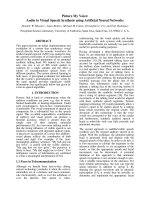
Fig. 1 Effect of the number of hidden neurons and number of cycles during training on the MSE, in the prediction of the capacity factor
(K0 ) for combination I. (a) 3D surface plot and (b) 3D contour plot.


HPLC optimization using ANNs

57

of the capacity factor (K0 ) of SAL and GUA to the changes in
pH (3.1–6.0) and mobile phase composition (18–42 methanol%), were emulated using a network of two inputs (pH
and methanol%), one hidden layer and two outputs (K0 for
SAL and GUA). For combination II, the behaviour of the separation factor (a) between ASC, PAR and between PAR,
GUA to the changes in pH (3.3–6.8) and mobile phase composition (20–90 methanol%), were emulated using a network of
two inputs (pH and methanol%), one hidden layer and two
outputs (a between ASC, PAR and between PAR, GUA).
Training data are listed in Tables 1 and 2 for combinations I
and II, respectively.
Neural networks were trained using different numbers of
neurons (2–20) in the hidden layer and training cycles (150–
500) for both combinations I and II. At the start of a training
run, weights were initialized with random values. During
training, modifications of the weights were made by backpropagation of the error until the error value for each

input/output data pair in the training data reached the predetermined error level. While the network was being

optimized, the testing data (Tables 1 and 2 for combinations
I and II, respectively) were fed into the network to evaluate
the trained net.
Multiple regression analysis
Multiple regression analysis (quadratic) was carried out using
STATISTICA software, release 5.0, 1995 (StatSoft Inc., USA).
Chromatographic experiments were performed in the pH
range of 3.1–6.0 or 3.3–6.8 and methanol% of 18–42% or
20–90% for combinations I and II, respectively. According
to these experimental data (Tables 1 and 2), model-fitting
methods gave the equations for the relationship between the
responses (K0 or a for combinations I and II, respectively)
and pH and mobile phase composition.

a

0.021
0.031
0.041
0.051
0.061
0.070
0.080
0.090
0.100
0.110
above

b
550

500
450

TRAINING

400
350
300
250
200
150
100

0

4

8

12

16

20

24

0.021
0.031
0.041

0.051
0.061
0.070
0.080
0.090
0.100
0.110

HIDDENN

Fig. 2 Effect of the number of hidden neurons and number of cycles during training on the MSE, in the prediction of the separation
factor (a), combination II. (a) 3D surface plot and (b) 3D contour plot.


58

M.A. Korany et al.
where p = methanol% and m = pH.
Results of the multiple regression analysis for both
combinations are summarized in Tables 3 and 4.

For combination I,
0

2

K ðSALÞ ¼ À3:538 À 0:552p À 6:688m þ 0:012p
À 0:079pm À 0:377m2

ð5Þ

Results and discussion

K0 ðGUAÞ ¼ 36:938 À 1:83p þ 0:178m þ 0:023p2
þ 0:01pm À 0:068m2

ð6Þ

For combination II,
a1 ðASC and PARÞ ¼ 41:944 þ 0:028p À 19:469m
þ 0:001p2 À 0:029pm þ 2:411m2

ð7Þ

Network topologies
The properties of the training data determine the number of input and output neurons. In this study, the number of factors
(pH and methanol%) forced the number of input neurons to
be two in both combinations. The number of responses including K0 of SAL and of GUA or a (ASC and PAR) and a (PAR

a2 ðPAR and GUAÞ ¼ 13:193 À 0:317p À 0:094m
þ 0:002p2 þ 0pm þ 0:014m2

ð8Þ

a

a

0.972
3.075
5.178

7.281
9.383
11.486
13.589
15.692
17.794
19.897
above

0.727
1.455
2.182
2.909
3.636
4.364
5.091
5.818
6.545
7.273
above

b

b

2.457
3.606
4.755
5.903
7.052

8.201
9.349
10.498
11.647
12.795
above

Fig. 3 Response surfaces for multifactor effect of pH and
methanol% on (a) capacity factor (K0 ) of salbutamol (SAL) and
(b) of guaiphenesin (GUA) generated by ANN with 12 hidden
neurons and 350 training cycles.

1.637
2.373
3.110
3.846
4.582
5.319
6.055
6.791
7.527
8.264
above

Fig. 4 Response surfaces for multifactor effect of pH and
methanol% on (a) separation factor between ascorbic acid and
paracetamol (a1) and (b) between paracetamol and guaiphenesin
(a2) generated by ANN with 14 hidden neurons and 250 training
cycles.

HPLC optimization using ANNs

59

a

a

2.002
3.602
5.202
6.801
8.401
10.001
11.601
13.201
14.800
16.400
above

0.526
1.273
2.021
2.768
3.515
4.263
5.010
5.758
6.505

7.253
above

b

b

2.535
3.677
4.819
5.961
7.104
8.246
9.388
10.530
11.672
12.814
above

Fig. 5 Response surfaces for multifactor effect of pH and
methanol% on (a) capacity factor (K0 ) of salbutamol (SAL) and
(b) of guaiphenesin (GUA) generated by REG model.

and GUA) for combinations I and II, respectively, forced the
number of output neurons also to be two.
The number of connections in the network is dependent
upon the number of neurons in the hidden layer. In the training phase, the information from the training data is transformed to weight values of the connections. Therefore, the
number of connections might have a significant effect on the
network performance. Since there are no theoretical principles
for choosing the proper network topology, several structures

were tested.
A problem in constructing the ANN was to find the optimal
number of hidden neurons. Another problem was over-fitting
or over-training, evident by an increase in the test error. Neural networks were trained using different numbers of hidden
neurons (2–20) and training cycles (150–500) for each combination. Neurons were added to the hidden layer two at a time.
The networks were trained and tested after each addition.

0.973
1.776
2.578
3.381
4.184
4.986
5.789
6.592
7.395
8.197
above

Fig. 6 Response surfaces for multifactor effect of pH and
methanol% on (a) separation factor between ascorbic acid and
paracetamol (a1) and (b) between paracetamol and guaiphenesin
(a2) generated by the REG model.

Since test set error is usually a better measure of performance
than training error, while the network has been optimized, test
data were fed through the network to evaluate the trained
network. After the addition of the 12th or the 14th hidden
neurons for combinations I and II, respectively, it became
evident that more hidden neurons did not improve the generalization ability of the network (Figs. 1 and 2).

Training of the networks
To compare the predictive power of the neural network structures, MSE was calculated for each model (with certain numbers of hidden neurons and training cycles). The performance
of the network on the testing data gives a reasonable estimate
of the network prediction ability.
The lowest testing MSE was obtained with 12 or 14 hidden
neurons and 350 or 250 training cycles for combinations I and
II, respectively (Figs. 1 and 2). After 350 or 250 cycles, extra


60

M.A. Korany et al.

training made the prediction ability worse and the test error began to increase. This effect is called over-training or over-fitting.
The combined effect of pH and methanol% on the capacity
factors or separation factors for combinations I and II,
respectively, generated by the best ANN model, are presented
in Figs. 3 and 4.
Multiple regression analysis
Eqs. (5) and (6) was used to predict K0 of SAL and GUA,
respectively, at any selected value for pH and methanol%.
Eqs. (7) and (8) could be also used to predict a (ASC and
PAR) and a (PAR and GUA), respectively, at any selected value for pH and methanol%. Predicted response surfaces drawn
from the fitted equations are shown in Figs. 5 and 6 for combinations I and II, respectively.

In studying the generalization ability of neural networks, five
additional experiments were performed (see Tables 5 and 6
for combinations I and II, respectively). In the experimental
points, the factor levels of the input variables were chosen so
that they were within the range of the original training data

24.0
38.0
35.0
40.0
35.0

a

c

To compare the predictive power of the regression model with
the neural network model, we compared experimental and predicted response factor values, mean of squares error (MSE),
average error percentage (Er%) and squared coefficients of
correlation (r2).

Method validation for the prediction of K0 of salbutamol (SAL) and guaiphenesin (GUA).

Methanol (%)

b

i¼1

where n is the number of experimental points, Ti is the measured (target) capacity factor or separation factor for combinations I and II, respectively, and Oi denotes the value predicted
by the model for a drug.
Comparison of the best network and the regression model

Method validation

Table 5

(interpolation). The generalization ability was studied by
consulting the network with test data and observing the
output values. The output values are hence predicted by the
network. This operation is called interrogating or querying
the model.
Average error percentage (Er%) is used for examination of
the best generalization ability or method validation of neural
networks (the smallest Er%).
(Er%) is calculated according to Eq. (9):
X
j½1 À ðOi =Ti ފj  100=n
ð9Þ
Er % ¼

pH

4.2
3.5
3.3
5.5
3.5

Predicted by ANNa

Measured

Predicted by REG

SAL

GUA

SAL

GUA

SAL

GUA

4.100
0.778
0.941
1.350
1.109

6.456
1.833
2.229
1.541
2.568

3.954
0.848
0.830
1.243
1.141

6.680
2.042
2.650
1.495
2.669

3.602
1.097
0.682
1.582
0.954

6.819
1.727
2.062
1.657
2.075

rb
r2
Er%c

0.989
0.978
0.070

0.997
0.994
0.051

0.966
0.932
0.223

0.992
0.983
0.115

ANN with 12 hidden neurons and 350 training cycles.
Coefficient of correlation.
Relative percentage error.

Table 6 Method validation for the prediction of the separation factors between ascorbic acid (ASC) and paracetamol (PAR), a1, and
between paracetamol (PAR) and guaiphenesin (GUA), a2.
Methanol (%)

70.0
44.0
25.0
30.0
90.0

a
b
c

pH

4.7
6.1

6.1
5.5
4.1

Measured

Predicted by ANNa

Predicted by REG

a1

a2

a1

a2

a1

a2

1.375
4.333
8.667
2.667
0.875

1.273
3.000

6.500
6.450
1.171

1.542
5.500
8.822
3.556
0.962

1.218
3.016
6.489
4.437
1.178

1.018
8.281
9.798
4.752
2.569

0.670
3.065
6.466
5.389
0.713

Rb
R2

ERR (%)c

0.893
0.596
0.168

0.915
0.837
0.048

0.900
0.953
0.804

0.810
0.910
0.181

ANN with 14 hidden neurons and 250 training cycles.
Coefficient of correlation.
Relative percentage error.


HPLC optimization using ANNs

61

4.5

4.5

(a)

4
3.5

Predicted value

3.5

3

K (SAL)

(a’)

4

2.5
2
1.5

3
2.5
2
1.5

1

1

0.5

0.5
0

0

1

2

3

4

0

5

1

2

8

4

5

8

(b)

7

(b’)

7

6

6

Predicted value

K (GUA)

3

Experimental value

Experimental point

5
4
3

5
4

3

2

2

1

1

0

0
1

2

3

4

5

0

Experimental point

Experimental value

ANN

2

4

6

8

Experimental value
Experimental value

REG

ANN

REG

Fig. 7 Capacity factors (a) of salbutamol (K0 SAL) and (b) of guaiphenesin (K0 GUA): experimental values, artificial neural network
estimated (ANN) and regression model estimated (REG).

In Fig. 7, experimental K0 of SAL and of GUA were compared with those predicted by ANN and with those calculated
by the regression models (Eqs. (5) and (6)). The ANN values
were closer to the experimental values than the REG values.
Fig. 8 also compared experimental a1 (ASC and PAR) and
a2 (PAR and GUA) with those predicted by ANN and with
those calculated by the regression models (Eqs. (7) and (8)).
The ANN values were closer to the experimental values than
the REG values.
The closeness of the data predicted by ANN compared

with REG is also illustrated by the validation graphs shown
in Figs. 7a0 , b0 and 8a0 , b0 where the former show little scatter around the experimental values compared with the REG
model.
In this sense, ANNs offer a superior alternative to classical
statistical methods. Classical ‘‘response surface modeling’’
(RSM) requires the specification of polynomial functions such
as linear, first order interaction, or second or quadratic, to undergo the regression. The number of terms in the polynomial is
limited to the number of experimental design points. On the
other hand, selection of the appropriate polynomial equation
can be extremely laborious because each response variable requires its own polynomial equation. The ANN methodology
provides a real alternative to the polynomial regression method as a means to identify the non-linear relationship. Using

ANNs, more complex relationships, especially nonlinear ones,
may be investigated without complicated equations.
ANN analysis is quite flexible concerning the amount and
form of the training data, which makes it possible to use more
informal experimental designs than with statistical approaches.
It is also presumed that neural network models might generalize better than regression models generated with the multiple
regression technique, since regression analyses are dependent
on pre-determined statistical significance levels. This means
that less significant terms are not included in the models.
The application of ANN is a totally different method, in which
all possible data are used for making the models more
accurate.
A possible explanation may be that in the regression model,
each solute has its own model. The neural network, however,
constructs one model for all solutes at all design points used
for training. In this way the information is obtained more completely as the peak sequence in the different chromatograms
can contribute to the model.
Conclusion

Neural networks proved to be a very powerful tool in HPLC
method development. The combined effect of pH and mobile
phase composition on the reversed-phase liquid chromato-


62

M.A. Korany et al.
12

12

(a)

(a’)

8

8

Predicted value

10

Alpha 1

10

6

4

6

4

2

2

0

0

1

2

3

4

0

5

2

Experimental point
7

6

6

8

10

7

(b)

(b’)

6

5

5
Predicted value

alpha 2

4

Experimental value

4
3

4
3

2

2

1

1
0

0
1

2

3

4

5

ANN

2

4

6

8

Experimental value

Experimental point
experimental value

0

REG

Experimental value

ANN

REG

Fig. 8 Separation factors (a) between ascorbic acid and paracetamol (a1), (b) between paracetamol and guaiphenesin (a2): experimental
values, artificial neural network estimated (ANN) and regression model estimated (REG).

graphic behavior of a mixture of salbutamol (SAL) and guaiphenesin (GUA), combination I, and a mixture of ascorbic
acid (ASC), paracetamol (PAR) and guaiphenesin (GUA),
combination II, was investigated. Results showed that it is possible to predict response factors more accurately using neural
networks than using regression models. An ANN method
was successfully applied to chromatographic separations for
modeling and process optimization. Moreover, neural network
models might have better predictive powers than regression
models. Regression analyses are dependent on pre-determined
statistical significance levels and less significant terms are usually not included in the model. With ANN methods, all data

are used potentially, making the models more accurate.

References
[1] Murtoniemi E, Yliruusi J, Kinnunen P, Merkku P, Leiviska¨ K.
The advantages by the use of neural networks in modelling the
fluidized
bed
granulation
process.
Int
J
Pharm
1994;108(2):155–64.

[2] Agatonovic Kustrin S, Zecevic M, Zivanovic LJ, Tucker IG.
Application of artificial neural networks in HPLC method
development. J Pharm Biomed Anal 1998;17(1):69–76.
[3] Boti VI, Sakkas VA, Albanis TA. An experimental design
approach employing artificial neural networks for the
determination of potential endocrine disruptors in food using
matrix
solid-phase
dispersion.
J
Chromatogr
A
2009;1216(9):1296–304.
[4] Piroonratana T, Wongseree W, Assawamakin A, Paulkhaolarn
N, Kanjanakorn C, Sirikong M, et al.. Classification of
haemoglobin typing chromatograms by neural networks and

decision trees for thalassaemia screening. Chemometr Intell Lab
Syst 2009;99(2):101–10.
[5] Khanmohammadi M, Garmarudi AB, Ghasemi K, Garrigues S,
de la Guardia M. Artificial neural network for quantitative
determination of total protein in yogurt by infrared
spectrometry. Microchem J 2009;91(1):47–52.
~ez Sede~
[6] Torrecilla JS, Mena ML, Ya´n
no P, Garci´a J. Field
determination of phenolic compounds in olive oil mill
wastewater by artificial neural network. Biochem Eng J
2008;38(2):171–9.
[7] Faur C, Cougnaud A, Dreyfus G, Le Cloirec P. Modelling the
breakthrough of activated carbon filters by pesticides in surface


HPLC optimization using ANNs
waters with static and recurrent neural networks. Chem Eng J
2008;145(1):7–15.
[8] Webb R, Doble P, Dawson M. Optimisation of HPLC gradient
separations using Artificial Neural Networks (ANNs):
application to benzodiazepines in post-mortem samples. J
Chromatogr B 2009;877(7):615–20.
[9] Tran ATK, Hyne RV, Pablo F, Day WR, Doble P.
Optimisation of the separation of herbicides by linear gradient
high performance liquid chromatography utilising artificial
neural networks. Talanta 2007;71(3):1268–75.
[10] Novotna´ K, Havlisˇ J, Havel J. Optimisation of high
performance
liquid

chromatography
separation
of
neuroprotective peptides: fractional experimental designs

63

[11]
[12]

[13]
[14]

combined with artificial neural networks. J Chromatogr A
2005;1096(1–2):50–7.
Miller JN, Miller JC. Statistics and chemometrics for analytical
chemistry. 4th ed. Prentice Hall; 2000.
Freeman JA, Skapura DM. Neural network algorithms: applications and programming techniques. Houston: Addison-Wesley;
1991.
Dayhoff JE. Neural network architectures: an introduction. New York: Van Nostrand Reinhold; 1990.
Lisbon
GJ.
Neural
network
current
applications. London: Chapman & Hall; 1992.