Summary of physics doctoral thesis: The role of hydrophobic and polar sequence on folding mechanisms of proteins and aggregation of peptides
Bạn đang xem bản rút gọn của tài liệu. Xem và tải ngay bản đầy đủ của tài liệu tại đây (3.31 MB, 33 trang )
MINISTRY OF EDUCATION
VIETNAM ACADEMY
AND TRAINING
OF SCIENCE AND TECHNOLOGY
GRADUATE UNIVERSITY SCIENCE AND TECHNOLOGY
———————
NGUYEN BA HUNG
THE ROLE OF HYDROPHOBIC AND POLAR SEQUENCE
ON FOLDING MECHANISMS OF PROTEINS AND
AGGREGATION OF PEPTIDES
Major: Theoretical and computational physics
Code: 9 44 01 03
SUMMARY OF PHYSICS DOCTORAL THESIS
HANOI − 2018
INTRODUCTION
The problem of protein folding has always been of prime concern in molecular
biology. Under normal physiological conditions, most proteins acquire well defined
compact three dimensional shapes, known as the native conformations, at which
they are biologically active. When proteins are unfolding or misfolding, they
not only lose their inherent biological activity but they can also aggregate into
insoluble fibrils structures called amyloids which are known to be involved in
many degenerative diseases like Alzheimer’s disease, Parkinson’s disease, type
2 diabetes, cerebral palsy, mad cow disease etc. Thus, determining the folded
structure and clarifying the mechanism of folding of the protein plays an important
role in our understanding of the living organism as well as the human health.
Protein aggregation and amyloid formation have also been studied extensively
in recent years. Studies have led to the hypothesis that amyloid is the general
state of all proteins and is the fundamental state of the system when proteins
can form intermolecular interactions. Thus, the tendency for aggregation and formation amyloid persists for all proteins and is a trend towards competition with
protein folding. However, experiments have also shown that possibility of aggregation and aggregation rates depend on solvent conditions and on the amino acid
sequence of proteins. Some studies have shown that small amino acid sequences
in the protein chain may have a significant effect on the aggregation ability. As
a result, knowledge about the link between amino acid sequence and possibility
of aggregation is essential for understanding amyloid-related diseases as well as
finding a way to treat them.
Although all-atom simulations are now widely used molecular biology, the
application of these methods in the study of protein folding problem is not feasible
due to the limits of computer speed. A suitable approach to the protein folding
problem is to use simple theoretical models. There are quite a number of models
with different ideas and levels of simplicity, but most notably the Go model and
the HP network model and tube model.
Considerations of tubular polymer suggest that tubular symmetry is a fundamental feature of protein molecules which forms the secondary structures of
proteins (α and β). Base on this idea, the tube model for the protein was developed by Hoang and Maritan’s team and proposed in 2004. The results of the
tube model suggest that this is a simple model and can describes well many of the
basic features of protein. The tube model is also the only current model that can
simultaneously be used for the study of both folding and aggregation processes.
1
In this thesis, we use a tube model to study the role of hydrophobic and
polar sequence on folding mechanism of proteins and aggregation of peptides.
Spatial fill of the tubular polymer and hydrogen bonds in the model play the
role of background interactions and are independent of the amino acid sequence.
The amino acid sequence we consider in the simplified model consists of two
types of amino acids, hydrophobic (H) and polar (P). To study the effect of HP
sequence on the folding process, we will compare the folding properties of the
tube model using the hydrophobic interaction (HP tube model) with tube model
using the pairing interaction which is similar to the Go model (Go tube model).
This comparison helps to clarify the role of non-native interactions in non-native
interactions. To study the role of the HP sequence on aggregation of protein, we
will compare the possibility of aggregation of peptide sequences with different HP
sequences including the consideration of the shape of the aggregation structures
and the properties of aggregation transition phase. In addition, in the study of
protein aggregation, we propose an improved model for hydrophobic interaction
in the tube model by taking into account the orientation of the side chains of
hydrophobic amino acids. Our research shows that this improved model allows
for obtaining highly ordered, long-chain aggregation structures like amyloid fibrils.
1. The objectives of the thesis:
The aim of the studies is to gain fundamental understanding of the role of
hydrophobic and polar sequence on folding mechanism of proteins and aggregation of peptides
2. The main contents of the thesis:
The general understanding of protein and protein folding, protein aggregation
is introduced in chapters 1, 2 of this thesis. Chapter 3 presents the methods
used to simulate and analyze the data. The obtained results of role of HP
sequence for protein folding are presented in chapter 4. The results of role of
HP sequence for protein aggregation are presented in chapter 5.
2
Chapter 1
Protein folding
1.1
Structural properties of proteins
Proteins are macromolecules that are synthesized in the cell and responsible
for the most basic and important aspects of life. Proteins are polymers (polypeptides) formed from sequences of 20 diffirent types of amino acids, the monomers
of the polymer. The amino acids in the protein differ only in their side chains
and are linked together through peptide bonds that form a linear sequence in a
particular order.
Under normal physiological conditions, most proteins acquire well defined
compact three dimensional shapes, knows as the native conformations, at which
they are biologically active.
The amino acid sequence in the protein determines the structure and function
of the protein. Proteins has four types of structure.
Primary structure: It is just the chemical sequence of amino acids along the
backbone of the protein. These amino acid in chain linked together by peptide
bonds.
Secondary structure is the spatial arrangement of amino acids. There are two
such types of structures: the α-helices and the β-sheets. This kind of structure
which maximize the number of hydrogen bonds (H-bonds) between the CO and
the NH groups of the backbone.
Tertiary structure: A compact packing of the secondary structures comprises
tertiary structures. Usually, theses are the full three dimensional structures of
proteins. Tertiary structures of large proteins are usually composed of several
domains.
Quaternary structure: Some proteins are composed of more than one polypeptide chain. The polypeptide chains may have identical or different amino acid
sequences depending on the protein. Each peptide is called a subunit and has its
own tertiary structure. The spatial arrangement of these subunits in the protein
is called quaternary structure
There are a number of semi-empirical interactions that are introduced by
chemists and physicists to describe interactions in proteins: disulfide bridges,
3
Coulomb interactions, Hydrogen bonds, Van der Waals interactions, Hydrophobic
interactions.
1.2
Protein folding phenomenon
Once translated by a ribosome, each polypeptide folds into its characteristic
three-dimensional structure from a random coil. Since the fold is maintained by a
network of interactions between amino acids in the polypeptide, the native state
of the protein chain is determined by the amino acid sequence (hypothesis of
thermodynamics).
1.3
Paradox of Levinthal
Levinthal paradox which addresses the question: how can proteins possibly
find their native state if the number of possible conformations of a polypeptide
chain is astronomically large?
1.4
Folding funnel
Based on theoretical and empirical research findings, Onuchic and his colleagues have come up with the idea of the folding funnel as depicted in Figure
1.1. The folding process of the protein in the funnel is the simultaneous reduction of both energy and entropy. As the protein begins to fold, the free energy
decreases and the number of configurations decreases (characterized by reduced
well width).
entropy
g
energy
folding
N
Figure 1.1: The diagram sketches of funnel describes the protein folding energy lanscape
4
Figure 1.2: Free energy lanscape in the two-state model. In this model, ∆F is the diference between the free
energy of the folded and unfolded states. ∆FN and , ∆FD , ∆F are the height of barrier from the unfolded and
folded states and free energy difference between the N and U states , respectively
In the canonical depiction of the folding funnel, the depth of the well represents the energetic stabilization of the native state versus the denatured state, and
the width of the well represents the conformational entropy of the system. The
surface outside the well is shown as relatively flat to represent the heterogeneity
of the random coil state.
1.5
The minimum frustration principle
The minimum frustration principle was introduced in 1989 by Bryngelson
and Wolynes based on spin glass theory. This principle holds that the amino acid
sequence of proteins in nature is optimized through natural selection so that the
frustrated caused by interaction in the natural state is minimal.
1.6
Two-state model for protein folding
Experimental observations suggest that the two-state model is a common
mechanism used to characterize folding dynamics of the majority of small, globuar
proteins. In a two-state model of protein folding, the single domain protein can
occupy only one of two states: the unfolded state (U) or the folded state (N).
The free energy diagram for two-state model is characterized by a large barrier
separating the folded state and the unfolded state corresponding minima of the
free energy of a reaction coordinate. The free energy difference between the N
and U states (∆F ) characterize the degree of stability of the folding state called
folding free energy. Rates of folding kf and unfolding ku obey the law Vant Hoff5
Arrhennius:
kf,u = ν0 exp −
∆FN,D
kB T
(1.1)
For ν0 is constant, T is the temperature and kB is the Boltzmann constant.
The change of such as temperature, pressure, and concentration may affect on the
∆F .
1.7
Cooperativity of protein folding
Cooperativity is a phenomenon displayed by systems involving identical or
near-identical elements, which act dependently of each other. The folding of
proteins is cooperative process. In the protein, cooperativity is applied to the twostate process and is understood as the sharpness of thermodynamic transitions.
In practice, cooperativity is determined by the parameter measured by the ratio
between the enthalpy van’t Hoff and the thermal enthalpy.
κ2 = ∆HvH /∆Hcal
(1.2)
High cooperativity means that the system satisfies the two-state standard and
κ2 is closer to 1, the higher the co-operation and vice versa.
1.8
Hydrophobic interaction
The hydrophobic effect is the observed tendency of nonpolar substances (such
as oil, fat) to aggregate in an aqueous solution and exclude water molecule. The
tendency of nonpolar molecules in a polar solvent (usually water) to interact with
one another is called the hydrophobic effect. In the case of protein folding, the
hydrophobic effect is important to understanding the structure of proteins. The
hydrophobic effect is considered to be the major driving force for the folding of
globular proteins. It results in the burial of the hydrophobic residues in the core
of the protein.
1.9
HP lattice model
In the HP lattice model, there are two types of amino acids with respect to
their hydrophobicity: polar (P), which tend to be exposed to the solvent on the
protein surface, and hydrophobic (H), which tend to be buried inside the globule
6
protein. The folding of the protein is defined as a random step in a 2D or 3D
network. Using this model, Dill had design some HP sequence that the minimal
energy state in the tight packet configurations was unique. The phase transition
of the sequences is designed to be well cooperative. Research shows that aggregate
due to hydrophobic interaction is the main driving force for folding.
1.10
Go model
The Go model ignores the specificity of amino acid sequences in the protein
chain and interaction potential is build based on the structure of the folded state.
The basis of the Go model is the maximum consistent principle of protein interactions in the folded state. The results of the study show that the Go model for the
folding mechanism is quite good with the experiment, especially in determining
the contribution of amino acid positions in the polypeptide chain to the transition state during protein folding. . Because the model is based on a native state
structure, the Go model can not predict the protein structure from the amino
acid sequence that is only used to study the folding process of a known structure.
1.11
Tube model
Considerations of symmetry and geometry lead to a description of the protein backbone as a thick polymer or a tube. At low temperatures, a homopolymer model as a short tube exhibits two conventional phases: a swollen essentially featureless phase and and a conventional compact phase, along with a novel
marginally compact phase in between with relatively few optimal structures made
up of α-helices and β-sheets. The tube model predicts the existence of a fixed
menu of folds determined by geometry, clarifies the role of the amino acid sequence in selecting the native-state structure from this menu, and explains the
propensity for amyloid formation.
7
Chapter 2
Amyloid Formation
2.1
The structure of amyloid fibril
(a)
(b)
Figure 2.1: 3D structure of the Alzheimer’s amyloid-β (1-42)fibrils has a PDB code of 2BEG (a) view along the
direction of fibril axis (b) view perpendicular to the direction of fibril axis
Amyloid fibrils possess a cross-β structure, in which β-strands are oriented
perpendicularly to the fibril axis and are assembled into β-sheets that run the
length of the fibrils (Figure 2.1). They generally comprise 24 protofilaments, that
often twist around each other. Repeated interactions between hydrophobic and
polar groups run along the fibril axis.
2.2
Mechanism of amyloid aggregation
The formation of amyloid can be considered to involve at least three steps
and are generally referred to as lag phase, growth phase (or elongation) phase
and an equilibration phase. Seeding involves the addition of a preformed fibrils to
a monomer solution thus increasing the rate of conversion to amyloid fibrils. Addition of seeds decreases the lag phase by eliminating the slow nucleation phase.
8
Chapter 3
Methods and Models for simulations
3.1
HP tube model
The backbone of the protein is models as a string of Cα atoms separated by
an interval of 3.8˚
A, forming a flexible tube of 2.5˚
A also has a constraint with both
the tube’s three radii (local and non-local). Potential 3 objects describing this
condition are given in figure 3.1)
Vtube (i, j, k) =
∞
0
if Rijk < ∆
if Rijk ≥ ∆
∀ i, j, k
(3.1)
The bending potential in the tube model is related to the spatial constraints of
the polypeptide chain. The bending potential at position i given by (Figure 3.1)
∞
Vbend (i) =
eR
0
if Ri−1,i,i+1 < ∆
if ∆ ≤ Ri−1,i,i+1 < 3.2 ˚
A
if Ri−1,i,i+1 ≥ 3.2 ˚
A.
(3.2)
eR = 0.3 > 0 and the unit corresponds to the energy of a local hydrogen
bond In the tube model, local hydrogen bonds are made up of atoms i and i+3 and
assigned to energy equal to − . Non-local hydrogen bonds are formed between the
atoms i and j > i + 4 and have the energy of −0.7 . The energy and geometric
constraints of a local hydrogen bond between the atom i and the atom j are
defined as follows:
j =i+3
ehbond = −
A ≤ rij ≤ 5.6 ˚
A
4.7 ˚
|bi · bj | > 0.8
|bj · cij | > 0.94
|bi · cij | > 0.94
(r
i,i+1 × ri+1,i+2 ) · ri+2,i+3 > 0 .
The same for a non-local hydrogen bond:
9
(3.3)
Local radius
of curvature
Non local radius
of curvature
Hydrophobic
interaction
Figure 3.1: Sketch of the potentials used in the tube model of the protein. r, y are the local radius of curvature,
nonlocal radius of curvature; z is distance between two amino acid residues; eR and eW are beding energy and
hydrophobic energy
j >i+4
ehbond = −0.7
4.1 ˚
A ≤ rij ≤ 5.3 ˚
A
|bi · bj | > 0.8
|bj · cij | > 0.94
|bi · cij | > 0.94 .
(3.4)
In the tube model, hydrophobic interactions are introduced in the form of paring
potential between non-continuous Cα atoms in sequence (j > i + 1) given by
Vhydrophobic (i, j) =
eW
0
rij ≤ 7.5 ˚
A
rij > 7.5 ˚
A,
(3.5)
eW denotes the hydrophobic interaction energy for each contact, depending
on the hydrophobicity of the amino acids i and j. In the most studies, these
values were selected by eHH = −0.5 , eHP = eP P = 0.
3.2
Go tube model
The Go tube model is a tube model in which hydrophobic interaction energy
is replaced by the same energy interaction as the Go-like interaction model:
E = Ebend + Ehbond + EGo .
(3.6)
Thus, the Go tube model retains the geometric and symmetric properties, the
10
bending energy and hydrogen bonds as in tube model. Go-type energy is built on
the structure of the given native state. Interactive Go is given by:
VGo (i, j) =
Cij eW
0
rij ≤ 7.5 ˚
A
rij > 7.5 ˚
A,
(3.7)
where Cij are the elements of the native contact map. Cij = 1 if between i
and j exist in the native state and Cij = 0 in the other case. An contact in the
native state is defined when the distance between two consecutive Cα atoms is
less than 7.5 ˚
A.
3.3
Tube Model with correlated side chain orientations
we apply an additional constraint on the hydrophobic contact by taking into
account the side chain orientation: ni · cij < 0.5 and −ni · cij < 0.5. Where ni
and nj are the normal vectors of the Frenet frames associated with bead i and
j, respectively, cij is an unit vector pointing from bead i to bead j. The new
constraint is in accordance with the statistics drawn from an analysis of PDB
structures
3.4
Structural protein parameters
To study the protein folding to the native state, we examine the properties
of the protein configurations obtained from the simulation through a number
of characteristic features including folding contacts, root mean square deviation
(rmsd) and radius of gyration (Rg ) .
3.5
Monte Carlo simulation method
For studying the folding and aggregation of protein, we carry out multiple independent Monte Carlo (MC) simulations with Metropolis algorithm. The transfer of states of the systems in the models used is made by pivot, crank-shaft
and tranlocation motion for protein aggregation and pivot, crank-shaft motion
for protein folding.
3.6
Parallel tempering
Parallel tempering , also known as replica exchange MCMC sampling, is a
simulation method aimed at improving the dynamic properties of Monte Carlo
11
method simulations of physical systems, and of Markov chain Monte Carlo (MCMC)
sampling methods more generally by exchanges configurations at different temperatures.
Using Metropolis algorithm to swap two configurations
kBA = min {1, exp [(βi − βj ) (Ei − Ej )]}
(3.8)
For kBA is the probability of moving from A to B. This method is very
effective to find the basic state simultaneously at each temperature still obtained
balanced set and they are easily applied on parallel computers.
3.7
The weighted histogram analysis method
The Weighted Histogram Analysis Method (WHAM) allows for optimal analysis of data obtained from MC simulations as well as other simulations over a
wide range of parameters by combining multiple histograms together.
The probability is found system at the temperature T
R
P (βk , E) =
Nk (E) e−βk E
l=1
(3.9)
R
nl exp [−βl E − fl ]
l=1
fk = ln
P (E, βk )
(3.10)
E
fm are calculated from Eqs. 3.9 and 3.10 self-consistently. Normally, fm
converge quickly when the histograms balance and overlap. Determining the
values of fk completely determines P (E, β) at any temperature.
12
Chapter 4
The role of hydrophobic and polar sequence on folding
mechanisms of proteins
In this chapter we study the folding process of protein in two models: the
HP tube Model and the Go tube Model. In this study, we construct the tube Go
model for the two strutures in such a way that the total hydrophobic energy of
each structure are the same in the two models. The study was conducted with
two proteins of the same length of N = 48: a three helix bundle (3HB) and a
GB1-like structure (GB1). Figure 4.1 shows the native state of protein GB1 and
3HB.
Figure 4.1: Ground state conformations of two HP sequences considered in our study: a three-helix bundle (a)
and a GB1-like structure (b)
In the HP tube model, eHH = −0.5 , eHP = eP P = 0 and the unit
sponds to the energy of a local hydrogen bond.
4.1
corre-
Thermodynamics of protein folding in HP tube model
Figure 4.2a–c show the temperature dependence of the averaged radius of
gyration, Rg , average energy E and the specific heat of 3HP protein in the HP
tube model. Average energy, radius decreases as the temperature decreases. The
specific heat graph has a maximum Cmax = 1526kB at Tf = 0, 296 /kB . It can
be seen that for the tube HP model there is a small shoulder on the right of
the specific heat peak at T ≈ 0.5 /kB corresponding to a sharp decrease in the
average radius of motion as the temperature decreases. At T ≈ 0.5 /kB there
is a sharp decrease in the size of the protein while the energy does not decrease
much.This shoulder corresponds to a collapse transition.
13
18
16
14
0.7 0.8
(b)
collapse
12
10
0.5 0.6
0.7 0.8
(c)
800
400
3HB
0.5 0.6
T(unitsofε/k B)
18
16
14
0.7 0.8
0.4 0.5
<E>(unitsofε)
-60
3HB
0.6 0.7
0.1 0.2 0.3
(e)
collapse
10
500
-40
GB1
12
600
1200
0
0.2 0.3 0.4
-40
8
0.1 0.2 0.3
C(unitsofkB)
1600
3HB
-30
0.1 0.2 0.3
8
0.2 0.3 0.4
C(unitsofkB)
0.5 0.6
<Rg>(Angstroms)
<Rg>(Angstroms)
0.2 0.3 0.4
-20
-20
GB1
0.4 0.5
(b)
14
12
10
8
0.1 0.2 0.3
0.6 0.7
(f)
4000
3HB
0.4 0.5
0
0.1 0.2 0.3
GB1
0.4 0.5
T(unitsofε/k B)
3HB
0.4 0.5
T(unitsofε/k B)
Figure 4.2: Temperature dependence of the averaged
radius of gyration, Rg , average energy E and the
specific heat of 3HP protein in the HP tube model
-40
GB1
0.6 0.7
20
18
0.4 0.5
(e)
16
14
12
10
8
0.1 0.2 0.3
GB1
0.4 0.5
0.6 0.7
(f)
1200
0
0.1 0.2 0.3
0.6 0.7
-30
1600
1000
100
-20
2000
(c)
2000
200
(d)
2400
3000
300
0
-10
0.1 0.2 0.3
0.6 0.7
5000
400
0.6 0.7
18
16
0.4 0.5
<Rg>(Angstroms)
3HB
folding
(a)
C(unitsofkB)
-60
0
<E>(unitsofε)
-40
-10
10
(d)
C(unitsofkB)
folding
0
<Rg>(Angstroms)
<E>(unitsofε)
<E>(unitsofε)
-20
10
(a)
0
0.6 0.7
800
400
0
0.1 0.2 0.3
GB1
0.4 0.5
0.6 0.7
T(unitsofε/k B)
Figure 4.3: similar as figure 4.2 in the tube Go model.
Same with GB1 protein (fig 4.2d–f), the transition temperature of the specific
heat maximum of GB1 protein is Tf = 0.243 /kB and maximum of the specific
heat Cmax = 509.7 kB , both significantly lower than 3HB, showing that the phase
transition of GB1 is less sharp and less cooperative.
4.2
Thermodynamics of protein folding in Go tube model
Figure 4.3 show the temperature dependence of the averaged energy E, average radius of gyration, Rg and the specific heat of 3HP and GB1 protein in
the Go tube model. The folding transition phase and collapse transition phase
are sharper than the HP tube model. For both proteins, the change of the average energy and the average radius of gyration were significantly greater at the
transition temperature with greater slope than the HP tube model. Specific heat
has only a single peak at the transition temperature Tf and in particular, no
shoulder appears at temperatures greater than the transition temperature. In the
tube Go model, the collapse and folding transitions coincide at temperature Tmax .
Collapse phase in the Go tube model is the same as the folding phase.
The folding transition temperature Tf is also slightly higher in the tube Go
model: 0.345 /kB versus 0.296 /kB for 3HB protein and 0.291 /kB versus 0.243
/kB for GB1 protein. The maximum of the specific heat,Cmax , are roughly 2.8
and 4.1 times higher in the tube Go model comparing to the tube HP model
corresponding to 3HB and GB1 protein (4269 kB versus 1526 kB for 3HB protein
and 2104 kB versus 509.7 kB for GB1 ). These observations suggest that the tube
14
Go model is significantly more cooperative than the tube HP model and the latter
also yields a higher stability of the native state.
Folding transition phase in HP tube model and Go tube model
(a)
-20
-10
(d)
E(unitsofε)
E(unitsofε)
4.3
-40
-60
(a)
(d)
-20
-30
-40
-50
5000
10000
15000
MCsteps(x105)
0
0.05 0.1
normalizedhistogram
0
12
(b)
10
rmsd(Angstroms)
rmsd(Angstroms)
0
(e)
8
6
4
2
0
0
5000
10000
15000
MCsteps(x105)
5000
10000
15000
MCsteps(x105)
(b)
12
0
0.03 0.06
normalizedhistogram
(e)
8
4
0
0
0.1
0.2
normalizedhistogram
0
5000
10000
15000
MCsteps(x105)
0
0.04
0.08
normalizedhistogram
(c)
(f)
Rg(Angstroms)
Rg(Angstroms)
12
10
8
(c)
12
(f)
10
8
6
0
5000
10000
15000
MCsteps(x105)
0 0.05 0.1 0.15
normalizedhistogram
0
E(unitsofε)
-40
-60
10000
15000
MCsteps(x105)
(b)
(e)
12
8
4
0
10000
15000
MCsteps(x105)
0 0.05 0.1 0.15
normalizedhistogram
(d)
-20
-40
0
16
5000
(a)
0
0
0.02
0.04
normalizedhistogram
rmsd(Angstroms)
rmsd(Angstroms)
5000
20
0
Rg(Angstroms)
(d)
-20
0
15000
Figure 4.5: Same as 4.4 but for GB1 in HP tube
model at Tf = 0.243 /kB
5000
10000
15000
MCsteps(x105)
0
0.03
0.06
normalizedhistogram
25
(b)
20
(e)
15
10
5
0
0
0.03 0.06
normalizedhistogram
0
5000
10000
15000
MCsteps(x105)
0
0.03
0.06
normalizedhistogram
28
24
(c)
(f)
Rg(Angstroms)
E(unitsofε)
(a)
10000
MCsteps(x105)
Figure 4.4: trajectories and normalized histograms of
3HB protien in HP tube model obtained at a large
time of 2 × 10⁹ MC steps at the folding transition
temperature Tf = 0.296 /kB
0
5000
20
16
12
8
0
5000
10000
MCsteps(x105)
15000
0
0.1
0.2
normalizedhistogram
(c)
24
20
16
12
8
0
5000
10000
MCsteps(x105)
Figure 4.6: Trajectories and normalized histograms
of 3HB protien in Go tube model obtained at a large
time of 2 × 10⁹ MC steps at the folding transition
temperature Tf = 0.345 /kB
(f)
15000
0 0.05 0.1 0.15
normalizedhistogram
Figure 4.7: Same as 4.6 but for GB1 in Go tube
model at Tf = 0.291 /kB
Figure 4.4 and figure 4.5 describes long trajectories 2 × 10⁹ MC steps at
15
temperature Tf = 0.296 /kB for 3HB protein and Tf = 0.243 /kB for GB1
protein in HP tube model. The energy and rmsd vary strongly at the transition
temperature, while the radius of gyration Rg is only around the median value.
Shows the existence of the folding phase at small energy and rmsd values, and
the denaturing phase at the energy values rmsd and large. For the 3HB protein,
the energy distribution graphs (Fig. 4.4(d)) and the root-mean-square deviation
(Figure 4.4(e)) have two peaks distinguish between folding and unfolding phase
and the radius gyration graph Rg has only one peak (Figure 4.4(f)). For GB1
proteins, the graphs of Rg have only one peak (Figure 4.5(f)) but the energy and
rmsd distribution graph has two peak (Figure 4.5(d,e)). These results indicate
that the existence of two phase: folding and unfolding phase for both proteins,
but the phase separation in terms of energy of 3HB is more apparent than that
of GB1. The phases of both proteins at tempature transition phase also did not
differ in average size shown by the radius of gyration. There are also intermediate
states between the two phases.
Figure 4.4 and figure 4.5 describes long trajectories 2 × 10⁹ MC steps at
temperature Tf = 0.345 /kB for GB1 protein and Tf = 0.345 /kB for GB1
protein in Go tube model. The energy, rmsd and Rg of the two proteins are
strongly variable over time. The energy state and rmsd diagram have two distinct
peak, the Rg histogram has a sharp peak at low values for folding state and broad
shoulders at large values. The two-phase separation: fold and unfold in the Go
tube model is much clearer than the HP tube model.
The effective free energy at a given temperature T is defined as F (E, rmsd) =
−kB T log P (E, rmsd). Here P (E, rmsd) is the density of the probability that the
protein is in the energy state E and rmsd given.
Figure 4.8 describes the free energy at T = Tf for the 3HB and GB1 proteins
in the HP tube model and the Go tube. In the Go tube model, free energy consists
of only two minimums showing the two states of phase transition. The HP tube
model has a more complex free energy surface, consisting of three minimums in
the case of 3HB proteins and 2 minima in the case of the GB1 protein. Basically,
the free energy surface of 3HB in the HP tube model still exhibits a 2-state
system due to the 2 minima of the unfold phase link together by a low margin
and can be lumped together. In all cases, there is always a free energy margin
between the folding and the unfolding phase. The unfolding phase of proteins in
the Go tube model is always high in energy, while unfolding phase in the HP tube
model involves energy states that range from low to high energy. The existence
of unfolding state with low energy is a consequence of the HP sequence in the
HP tube model, allowing the formation of hydrophobic contacts that do not exist
16
(a)
10
(b)
14
Tube HP model: 3HB
9
8
11
6
Rmsd
Rmsd
13
12
12
10
11
12
7
8
10
9
6
9
8
4
10
5
4
3
7
2
8
2
7
6
1
-70
Tube Go model: 3HB
14
13
-60
-50
-40
-30
0
-70
-20
-60
-50
-40
E
-20
-10
0
E
(c)
11
-30
(d)
16
Tube HP model: GB1
Tube Go model: GB1
12
10
14
14
13
9
11
12
8
12
10
10
Rmsd
Rmsd
7
6
9
5
11
8
10
6
9
4
8
2
2
1
-40
4
8
3
7
-35
-30
-25
-20
-15
-10
7
0
-5
E
-50
-40
-30
E
-20
-10
0
Figure 4.8: Two-dimensional free energy landscape as the function of E and rmsd at the folding transition
temperature Tf = 0.345 /kB in HP tube model (a), Tf = 0.296 /kB in Go tube model (b) for 3HB protien
and at Tf = 0.291 /kB in HP tube model (c), Tf = 0.243 /kB in Go tube model (d) for GB1 protein
in the native state. At the same time, the folding transition temperature Tf in
the HP tube model lower in the Go model also makes it easier to form hydrogen
bonds in the unfolded state.
Comparison of the HP tube model and the Go tube model suggests that
changing the model changes the transition state. Specifically, for the 3HB protein, the transition state is near the (E, rmsd) = (−43 , 5.5˚
A) in HP tube model,
and (−24 , 5˚
A) in Go tube model. For GB1 protein, the transition state is near
(−26 , 5.8˚
A) in the HP tube model and (−28 , 8˚
A) in the Go tube model. However, it can be seen that the transition state is not as great as the change of
unfolded status when moving from the HP tube model to the Go tube model.
This is consistent with previous theoretical and empirical studies suggesting that
the mechanism of protein folding as well as the transition state depends primarily
on the geometry of the folded state.
4.4
Effect of hydrophobic interaction intensity on folding process
3HB protein continued to be used in this study. The value eHH varies from
0.15 to 0.7. Fig 4.10 describes the eHH dependence of the specific heat. When eHH
increases, Cmax decreases, Tf increases. The graphs have a sharp peak signaling
17
εHH=-0.70
εHH=-0.50
20
εHH=-0.30
εHH=-0.21
εHH=-0.20
εHH=-0.19
(b)
Rg (units of A0)
18
(c)
16
14
12
10
8
(a)
(d)
0.2
(e)
Figure 4.9: Ground state conformations obtained by
the simulations for 3HB protein with varying hydrophobic interaction intensities. The display structure corresponds to eHH = −0.2 (a), eHH = −0.21
(b), eHH = −0.3 (c), eHH = −0.5 (d), eHH =
−0.7 (e).
0.3
0.4
0.5
T (units of ε/kB)
0.6
0.7
Figure 4.10: Temperature dependence of the specific
heat of 3HP protein in the HP tube model with different hydrophobic interaction intensities eHH = −0.2 ,
−0.3 , −0.5 v −0.7 .
the phase transition type 1. From eHH = −0.3 to eHH = −0.7 graph has a small
shoulder, it expands when eHH increases. At the values |eHH | < 0.3 epsilon the
shoulder does not exist or very small to be recognized on the graph.
4.11 depicts the dependence of the average energy E and the radius of gyration Rg on the temperature. Average energy changes at the folding transition
temperature Tf . When |eHH | > 0.2 , then the change of Rg by the temperature
is monotonous. The change of Rg by temperature occurs more slowly and the inflection point of the graph occurs at higher temperatures as |eHH | increases. This
proves that as |eHH | increases, the collapse phase occurs at higher temperatures.
For |eHH | ≤ 0.2 , the radius of the radius depends on temperature in the form of
non-monotonous: at low temperature Rg has a large value corresponding to the
basic state is single-α; as the temperature rises, the single helix becomes unstable
due to thermal oscillations and therefore Rg decreases; As temperatures continue
to rise, the hydrogen bonds break down and the protein configuration is folded in
size increasing lead the Rg increase.
The cooperativity depend on the hydrophobic force intensity is determined
by the ratio between the enthalpy van’t Hoff and the thermal enthalpy κ2 =
∆H vH /∆Hcal . The value κ2 equal to 0, 5975 ± 0, 0166; 0, 6181 ± 0, 0116; 0, 7267 ±
0, 0206; 0, 7475 ± 0, 0256 for HH = 0, 2; 0, 3; 0, 5; 0, 7. The results show that when
the hydrophobic interaction is stronger, the cooperation also becomes stronger
show by the increasing of the value of κ2 .
18
<E>(unitsofε)
20
0
-20
-40
(a)
-80
-100
0.2
0.3
22
0.4
0.5
eHH=-0.19
eHH=-0.20
20
<Rg>(Angstroms)
eHH=-0.19
eHH=-0.20
eHH=-0.21
eHH=-0.30
eHH=-0.50
eHH=-0.70
-60
0.6
0.7
eHH=-0.21
eHH=-0.30
0.8
0.9
1
eHH=-0.50
eHH=-0.70
18
16
(b)
14
12
10
8
0.2
0.3
0.4
0.5
0.6
0.7
0.8
0.9
1
T(unitsofε/k B)
Figure 4.11: Temperature dependence of the average energy E (a), the averaged radius of gyration, Rg (b)
of 3HP protein in the HP tube model with different hydrophobic interaction intensities eHH = −0.2 , −0.3 ,
−0.5 v −0.7 .
19
Chapter 5
the role of hydrophobic and polar sequence on
aggregation of peptides
This chapter studies the aggregation of the short peptide in the tube model
with correlated side chain orientations. We study the role of the HP sequence on
protein aggregation and formation of amyloid fibrils. We consider 12 HP sequences
of length N = 8 as given in table 5.1 with number of peptide in each systems
changing from m = 1 to m = 20. The sequences, denoted as S1 through S12, are
selected in such a way that they contain only 2 or 3 hydrophobic (H) residues,
corresponding to hydrophobic fraction of 25% and 37.5%, respectively. Figure 5.1
shows that the lowest energy conformation obtained in the simulations,supposed
to be the ground state of a given system, strongly depends on the sequence.
5.1
Sequence dependence of aggregate structures
Fig. 5.1 shows that the lowest energy conformation obtained in the simulations. Two sequences, S2 and S11, form a double layer β-sheet structure with
characteristics similar to that of a cross-β structure. A similar structure but less
fibril-like is also found for sequence S12 with some parts that are non-β-sheet.
Both sequences S3 and S4 form a α-helix bundle. The helix bundle of sequence
S4 however is more ordered and has an approximate cylinder shape, in which the
α-helices are almost parallel to each other.
The role of hydrophobic residues in aggregation can be figured out from the
structures of the aggregates. The packing of hydrophobic side chains is best
Table 5.1: HP sequences of amino acids of peptides considered in present study (H – hydrophobic, P – polar).
The parameter s denotes the minimal sequence separation between two consecutive H amino acids.
Sequence name
S1
S2
S3
S4
S5
S6
S7
S8
S9
S10
S11
S12
Sequence
PPPHHPPP
PPHPHPPP
PPHPPHPP
PHPPPHPP
PHPPPPHP
HPPPPPHP
HPPPPPPH
PPHHHPPP
PPHPHHPP
PHPPHHPP
PHPHPHPP
PHPPHPHP
20
s
1
2
3
4
5
6
7
1
1
1
2
2
S1
S2
S3
S4
S5
S6
S7
S8
S9
S10
S11
S12
Figure 5.1: Ground state conformations obtained by the simulations for systems of M = 10 peptides for 10 HP
sequences (S1–S10) as given in Table 5.1.
observed for sequences S2 and S11, for which the hydrophobic residues are aligned
within each β-sheet and the hydrophobic side chains from the two β-sheets are
facing each other. This packing is possible due to the HPH pattern in these
sequences which position the hydrophobic side chains on one side of each β-sheet.
An alignment of hydrophobic residues is also seen for sequence S12 due to the
HPH segment of this sequence. In the aggregate of sequences S4, which is a helix
bundle, the hydrophobic side chains are gathered along the bundle axis, thanks to
to the alignment of hydrophobic side chains along one side of each α-helix. This
alignment is due to the HPPPH pattern in the S4 sequence. On the other hand,
the S3 sequence with the HPPH pattern also forms a helix but the hydrophobic
side chains are not well aligned in the helix, leading to a less ordered aggregate.
5.2
Thermodynamics of aggregation
We find that the specific heat strongly depends on both the sequence and
the system size. Fig. 5.2 and Fig. 5.3 show the temperature dependence of
the specific heat per molecule for various system sizes for sequences S2 and S4,
respectively. For sequence S2, it is shown that as M increases the specific heat’s
peak shifts toward higher temperature and its height increases (Fig. 5.2). This
result indicates that the aggregate becomes increasingly stable and the transition
becomes more cooperative as the system size increases. For sequence S4, for
which the aggregates are helix bundles, the height of the main peak increases
with M but the position of the peak varies non-monotonically (Fig. 5.3). Note
that the aggregation transition for sequences S4 is always found at a slightly lower
temperature than the folding transition of individual chain. This is in contrast
21
M=1
M=2
C/M (kB)
1000
M=4
M=5
M=1
1000
M=1
M=2
M=3
M=4
M=5
M=6
M=8
M=10
S2
M=6
M=2
M=6
M=1
M=2
M=4
M=6
M=10
S4
100
100
10
M=8
10
T*
T*
1
0.14
M=4
C/M (kB)
10000
M=3
M=10
1
0.16
0.18
0.2
0.22
0.24
0.26
0.1 0.12 0.14 0.16 0.18 0.2 0.22 0.24 0.26
T (ε/kB)
T (ε/kB)
M=10
Figure 5.2: Temperature dependence of the specific Figure 5.3: Same as Fig. 5.2 but for sequence S4
heat C per molecule for sequence S2 systems with the systems at 1 mM concentration. For clarity, the system
number of chains M equal to 1, 2, 3, 4, 5, 6, 8 and 10 sizes shown are fewer than for sequences S2.
as indicated. The position of a putative physiological
temperature, T ∗ , is indicated.
with sequence S2, whose aggregation transition temperature is always higher than
the folding temperature of a single chain.
In Fig. 5.4, the results of the maximum specific heat per molecule, Cpeak /M ,
and the temperature of the peak, Tpeak , are combined for all sequences considered
and for several values of M . It is shown that the variation of both Cpeak /M
and Tpeak increases with M . Note that for M = 10, the highest specific heat
maxima correspond to sequences S2 and S11 whose aggregates are fibril-like (see
Fig. 5.1). For sequences S2 and S11, Cpeak /M is not only the highest among
all sequences but also increases with M much faster than other sequences. Our
results indicates that the propensity of forming fibril-like aggregates is associated
with the cooperativity of the aggregation transition.
The wide variation in the transition temperatures Tpeak among sequences suggests another interesting aspect of aggregation. Suppose that we consider the systems at the physiological temperature, T ∗ . In our model, a rough estimate of T ∗
could be 0.2 /kB , which corresponds to a local hydrogen bond energy of 5 kB T ∗ .
For M = 1, one finds that all sequences but S10 has Tpeak < T ∗ suggesting that
the peptides are substantially unstructured at T ∗ as a single chain. For M = 6
and M = 10, only three sequences, S3, S4 and S5, have Tpeak < T ∗ , while the
other have Tpeak > T ∗ . Thus, sequences S3, S4 and S5 do not aggregate at T ∗
while other sequences do. This result indicates that the variation of aggregation
transition temperatures among sequences is also a reason why protein sequences
behave differently towards aggregation at the physiological temperature. Some se22
quences do not aggregate because aggregation is thermodynamically unfavorable
at this temperature.
Note that the ability of forming fibril-like aggregates is not necessarily associated with a high aggregation transition temperature. In fact, Fig. 5.4b shows
that sequences S2 and S11 have only a medium value of Tpeak among all sequences,
for both M = 6 and M = 10. Some sequences with a higher Tpeak , such as S8, S9
and S10, form disordered aggregates.
(a)
Cpeak/M (units of kB)
2500
M=10
M=6
M=1
2000
1500
1000
5
500
0
0
(b)
2
3
4
5
6
7
8
9
10
11
12
E (units of ε)
1
Tpeak (units of ε/kB)
0.4
0.36
0.32
0.28
0.24
-5
-10
S2, M=4
-15
T=0.2
-20
T*
0.2
-25
0.16
0
1
2
3
4
5
6
7
8
9
10
11
12
100
200
300
400
500
600
MC steps (x106)
sequence #
Figure 5.4: Dependence of the maximum of the spe- Figure 5.5: Energy as function of Monte Carlo steps in
cific heat Cpeak per molecule (a) and its temperature a trajectory at T = 0.2 for the sequence S2 system with
Tpeak (b) on the sequence for systems of M = 10 (solid), M = 4 at 1 mM concentration. The conformation shown
M = 6 (dashed) and M = 1 (dotted) peptides at 1 mM is a metastable state with a 3-peptide β-sheet in contact
concentration. The horizontal line in (b) indicates a pu- with a disordered helix formed by the 4th peptide.
tative physiological temperature T ∗ .
Fig. 5.2 shows that for sequence S2, systems of M ≤ 4 have the specific
heat peaked at a lower temperature than T ∗ = 0.2 /kB , which means that these
systems do not aggregate at T ∗ . Only for M > 4, the specific heat peak temperature is higher than T ∗ indicating that the fibril-like aggregates formed by this
sequence are stable at T ∗ . Thus, a sufficient number of peptides is needed for the
aggregation to happen at a given temperature. We also find that the lower peak
in the specific heat of the system of M = 4 (Fig. 5.2) corresponds to a transition
from metastable aggregates at intermediate temperature to the ground state at
low temperature.
Fig. 5.5 shows the trajectory of an equilibrium simulation at T = 0.2 /kB for
sequences S2 with M = 4. The time dependence of the system’s energy in this
trajectory indicates that the peptides do not aggregate most of the time, so that
the energy is relatively high, but for some short periods they can spontaneously
23
form a metastable aggregate of a much lower energy. This metastable aggregate
has a three-stranded β-sheet (Fig. 5.5, inset) and could act as a template for fibril
growth in systems of more peptides.
5.3
Kinetics of fibril formation
First, we consider a system of M = 10 peptides with concentration c = 1
mM under equilibrium condition. Fig. 5.6 shows the dependence of the total
free energy of the system on the size of the largest aggregate, m, formed at three
temperatures slightly below Tpeak including T = T ∗ = 0.2 /kB . It is shown that
for all these temperatures the free energy has a maximum at m = 3, suggesting
that m = 3 could be the size of the critical nucleus for fibril formation. The free
energy barrier for aggregation in Fig. 5.6 is found to increase with T and is about
of 1 kB T to 4 kB T . This barrier is not large and is consistent with the fact that
the sequence considered is highly aggregation-prone. For m > 3, Fig. 5.6 shows
that the free energy decreases almost linearly with n, which is consistent with the
fact that the growth of the aggregate in size is essentially one-dimensional.
We then considered a larger system of M = 20 peptides and studied the
time evolutions from random configurations of dispersed monomers. Up to 100
independent trajectories are carried out to determine the statistics. We first
consider the system at concentration c = 1 mM and T = 0.2 /kB . Fig.5.7 (a
and b) shows three typical trajectories with the total energy E and the size of
the largest aggregate m as functions of time. Interestingly, these trajectories
show clear evidence of an initial lag time, during which m fluctuates but remains
small (m ≤ 3) before a rapid and almost monotonic growth (Fig. 5.7 b). They
also shows that nucleation is complete for m = 3. A peptide configuration at
a nucleation event is shown on Fig. 5.7d indicating that a possible nucleus is a
three-stranded β-sheet formed by three peptides (Fig. 5.7e). Fig. 5.7c shows that
the system can form multiple aggregates of various sizes. The distribution of the
aggregate size obtained after a sufficient long time is bimodal reflecting the fact
that the system size is finite and clusters of less than 4 peptides are unstable.
Thus, one either observes one large cluster with size close to the system size or
several smaller clusters. The largest aggregates of m = 20 peptides have the form
of an elongated double β-sheet strongly resemble a cross-β-structure (Fig. 5.7f).
It is shown in Fig. 5.8 (a and b) that for T = 0.2 /kB , the time dependence
of nβ can be fitted well to the exponential relaxation function of M (1 − e−t/t0 ),
where t0 is the characteristic time of aggregation. This time dependence also
depends strongly on the concentration c with t0 increases more than 3 times by
24