Maximum entropy approach to portfolio optimization: Economic justification of an intuitive diversity idea
Bạn đang xem bản rút gọn của tài liệu. Xem và tải ngay bản đầy đủ của tài liệu tại đây (844.87 KB, 12 trang )
Asian Journal of Economics and Banking (2019), 3(2), 17–28
17
Asian Journal of Economics and Banking
ISSN 2588-1396
/>
Maximum Entropy Approach to Portfolio
Optimization: Economic Justification
of an Intuitive Diversity Idea
Laxman Bokati1 , Vladik Kreinovich2 ❸
1 Computational
2 University
Science Program, 500 W. University
of Texas at El Paso, El Paso, TX 79968, USA
Article Info
Abstract
Received: 25/02/2019
Accepted: 01/08/2019
Available online: In Press
The traditional Markowitz approach to portfolio
optimization assumes that we know the means,
variances, and covariances of the return rates of
all the financial instruments. In some practical
situations, however, we do not have enough information to determine the variances and covariances, we only know the means. To provide a
reasonable portfolio allocation for such cases, researchers proposed a heuristic maximum entropy
approach. In this paper, we provide an economic
justification for this heuristic idea.
Keywords
Portfolio Optimization, Maximum Entropy Approach
JEL classification
C58, G11, C440
MSC2010 classification
62P20, 91B80, 91B24, 90B50,
94A17
❸
Corresponding author: Vladik Kreinovich, University of Texas at El Paso, TX 79968, USA.
Email address:
18
Laxman Bokati, Vladik Kreinovich/Maximum Entropy Approach to...
1 FORMULATION
PROBLEM
OF
THE
Portfolio optimization:
general
problem. What is the best way to
invest money? Usually, there are several possible financial instruments; let
us denote the number of available financial instruments by n. The questions
is then: what portion wi of the overall money amount should we allocate to
each instrument i? Of course, these portions must be non-negative and add up
to one:
n
wi = 1.
(1)
i=1
The corresponding tuple w
=
(w1 , . . . , wn ) is known as an investment
portfolio, or simply portfolio, for short.
Case of complete knowledge:
Markowitz solution. If we place
money in a bank, we get a guaranteed
interest, with a given rate of return r.
However, for most other financial instruments i, the rate of return ri is not
fixed, it changes (e.g., fluctuates) year
after year. For each values of instrument returns, the corresponding portfon
w i · ri .
lio return r is equal to r =
i=1
In many practical situations, we
know, from experience, the probabilistic distributions of the corresponding
rates of return. Based on this past
experience, for each instrument i, we
can estimate the expected rate of return
µi = E[ri ] and the corresponding standard deviation σi = E[(ri − µi )2 ]. We
can also estimate, for each pair of financial instruments i and j, the covariance
def
cik = E[(ri − µi ) · (rj − µj )].
By using this information, for each
possible portfolio w = (w1 , . . . , wn ), we
can compute the expected return
n
w i · µi
µ = E[r] =
(2)
i=1
and the corresponding variance
n
n
2
n
wi2 ·σi2 +
σ =
i=1
cij ·wi ·wj . (3)
i=1 j=1
The larger the expected rate of return µ we want, the largest the risk that
we have to take, and thus, the larger
the variance. It is therefore reasonable,
given the desired expected rate of return µ, to find the portfolio that minimizes the variance, i.e., that minimizes
the expression (3) under the constraints
(1) and (2).
This problem was first considered
by the future Nobelist Markowitz,
who proposed an explicit solution to
this problem; see, e.g.,[8]. Namely, the
Lagrange multiplier method enables
to reduce this constraint optimization problem to the following unconstrained optimization problem: minimize the expression
n
n
wi2
·
σi2
n
cij · wi · wj
+
i=1
i=1 j=1
n
+λ1 ·
wi − 1
i=1
n
+λ2 ·
w i · µi − µ
(4)
i=1
where λ1 and λ2 are Lagrange multipliers that need to be determined from the
conditions (1) and (2).
Asian Journal of Economics and Banking (2019), 3(2), 17-28
Differentiating the expression (4) by
the unknowns wi , we get the following
system of linear equations:
2σi · wi + 2
cij · wj + λ1 + λ2 · µi = 0.
j=i
(5)
Thus,
(1)
(2)
wi = λ1 · wi + λ2 · wi ,
(6)
(j)
where wi are solutions to the following
systems of linear equations
2σi · wi + 2
cij · wj = −1
(7)
cij · wj = −µi .
(8)
j=i
and
2σi · wi + 2
j=i
Substituting the expression (6) into
the equations (1) and (2), we get a system two linear equations for two unknowns λ1 and λ2 . From this system,
we can easily find the coefficients λi and
thus, the desired portfolio (6).
Case of complete information:
modifications of Markowitz solution. Some researchers argue that variance may be not the best way to describe the intuitive notion of risk. Instead, they propose to use other statistical characteristics, e.g., the quantile qα
corresponding to a certain small probability α – i.e., a value for which the
probability that the returns are very low
(r ≤ qα ) is equal to α.
Instead of the original Markowitz
problem, we thus have a problem of
maximizing qα – or another characteristic – under the given expected return
µ. Computationally, the resulting constraint optimization problems are no
19
longer quadratic and thus, more complex to solve, but they are still well formulated and thus, solvable.
Case of partial information: formulation of the general problem. In
many practical situations, we only have
partial information about the probabilities of different rates of return ri .
For example, in some cases, we
know the expected returns µi , but we
do not have any information about the
standard deviations and covariances.
What portfolio should we select in such
situations?
Maximum Entropy approach: reminder.
Situations in which we
only have partial information about the
probabilities – and thus, several different probability distributions are consistent with the available information –
such situations are ubiquitous.
Usually, some of the consistent distributions are more precise, some are
more uncertain. We do not want to pretend that we know more than we actually do, so in such situations of uncertainty, a natural idea is to select a distribution which has the largest possible
degree of uncertainty. A reasonable way
to describe the uncertainty of a probability distribution with the probability
density ρ(x) is by its entropy
✂
S=−
ρ(x) · ln(ρ(x)) dx.
(9)
So, we select the distribution whose
entropy is the largest; see, e.g., [5].
In many cases, this Maximum Entropy approach makes perfect sense. For
example, if the only information that we
have about a probability distribution is
that it is located on an interval [x, x],
then out of all possible distributions, the
20
Laxman Bokati, Vladik Kreinovich/Maximum Entropy Approach to...
Maximum Entropy approach selects the
uniform distribution ρ(x) = const on
this interval. This makes perfect sense –
if we do not have any reason to believe
that one of the values from the interval is more probable than other values,
then it makes sense to assume that all
the values from this interval are equally
probable, which is exactly ρ(x) = const.
In situations when we know
marginal distributions of each of the
variables, but we do not have any information about the dependence between
these variables, the Maximum Entropy
approach concludes that these variables
are independent. This also makes perfect sense: if we have no reason to believe that the variables are positively or
negatively correlated, it makes sense to
assume that they are not correlated at
all.
If all we know is the mean and the
standard deviation, then the Maximum
Entropy approach leads to the normal
(Gaussian) distribution – which is in
good accordance with the fact that such
distributions are indeed ubiquitous.
So, in situations when we only have
a partial information about the probabilities of different return values, it
makes sense to select, out of all possible
probability distributions, the one with
the largest entropy, and then use this
selected distribution to find the corresponding portfolio.
Problem: Maximum Entropy approach is not applicable to the case
when only know µi . In many practical situations, the Maximum Entropy
approach leads to reasonable results.
However, it is not applicable to the situation when we only know the expected
rates of return µi .
This impossibility can be illustrated
already on the case when we have a single financial instrument. Its rate of return r1 can take any value, positive or
negative, the only information that we
have about the corresponding probability distribution ρ(x) is that
✂
µ1 =
x · ρ(x) dx
(10)
and, of course, that ρ(x) is a probability
distribution, i.e., that
✂
ρ(x) dx = 1.
(11)
The constraint optimization problem of maximizing the entropy (9) under the constraints (10) and (11) can be
reduced to the following unconstrained
optimization problem: maximize
✂
−
ρ(x) · ln(ρ(x))dx
✂
x · ρ(x)dx − µ1
+λ1 ·
✂
+λ2 ·
ρ(x)dx − 1 ,
(12)
Differentiating the expression (12)
with respect to the unknown ρ(x) and
equating the derivative to 0, we get
− ln(ρ(x)) − 1 + λ1 · x + λ2 = 0,
hence
ln(ρ(x)) = (λ2 − 1) + λ1 · x
and ρ(x) = C · exp(λ1 · x), where C =
exp(λ2 − 1). The problem is that the integral of this exponential function over
the real line is always infinite, we cannot get it to be equal to 1 – which means
Asian Journal of Economics and Banking (2019), 3(2), 17-28
that it is not possible to attain the maximum, entropy can be as large as we
want.
So how do we select a portfolio in
such a situation?
A heuristic idea. In the situation
in which we only know the means µi ,
we cannot use the Maximum Entropy
approach to find the most appropriate
probability distribution. However, here,
the portions wi – since they add up to
1 – can also be viewed as kind of probabilities. It therefore makes sense to look
for a portfolio for which the corresponding entropy
n
−
wi · ln(wi )
(13)
i=1
attains the largest possible value under
the constraints (1) and (2); see, e.g.,
[1, 3, 9, 10, 11, 12].
This heuristic idea sometimes leads
to reasonable results. Here, entropy can
be viewed as a measure of diversity.
Thus, the idea to bring more diversity
to one’s portfolio makes perfect sense.
However, there is a problem.
Remaining
problem. The problem
is that while the weights wi do add
up to one, they are not probabilities. So,
in contrast to the probabilistic case, where
the Maximum Entropy approach has
many justifications, for the weights,
there does not seem to be any reasonable justification. It is therefore desirable to either justify this heuristic
method - or provide a justified alternative.
What we do in this paper. In this
paper, we provide a justification for the
Maximum Entropy approach. We also
show that a similar idea can be applied
21
to a slightly more complex – and more
realistic – case, when we only know
bounds µi and µi on the values µi .
2 CASE WHEN WE ONLY
KNOW
THE
EXPECTED
RATES OF RETURN µi : ECONOMIC JUSTIFICATION OF
THE MAXIMUM ENTROPY
APPROACH
General definition. We want, given n
expected return rates µ1 , . . . , µn , to generate the weights w1 = fn1 (µ1 , . . . , µn ),
. . . , wn = fnn (µ1 , . . . , µn ) depending on
µi for which the sum of the weights is
equal to 1.
Definition 1. By a portfolio allocation
scheme, we mean a family of functions
fni (µ1 , . . . , µn ) = 0 of non-negative
variables µi , where n is arbitrary integer larger than 1, and i = 1, 2, . . . , n,
such that for all n and for all µi ≥ 0,
we have
n
fni (µ1 , . . . , µn ) = 1.
i=1
Symmetry. Of course, the portfolio allocation should not depend on the order
in which we list the instrument.
Definition 2. We say that a portfolio allocation scheme is symmetric if for
each n, for each µ1 , . . . , µn , for each
i ≤ n, and for each permutation π :
{1, . . . , n} → {1, . . . , n}, we have
fni (µ1 , . . . , µn ) = fn,π(i) (µπ(1) , . . . , µπ(n) ).
Pairwise comparison. If we only have
two financial instruments (n = 2) with
22
Laxman Bokati, Vladik Kreinovich/Maximum Entropy Approach to...
expected rates µ1 and µ2 , then we assign weights w1 and w2 = 1 − w1 depending on the known values µ1 and µ2 :
w1 = f21 (µ1 , µ2 ) and w2 = f22 (µ1 , µ2 ).
In the general case, if we have n instruments including these two, then the
amount fn1 (µ1 , . . . , µn )+fn2 (µ1 , . . . , µn )
is allocated for these two instruments.
Once this amount is decided on, we
should divide it optimally between these
two instruments. The optimal division
means that the first instrument gets
the portion f21 (w1 , w2 ) of this overall
amount, so we must have
to show that every symmetric and consistent portfolio allocation scheme has
the form (16).
Indeed, let us assume that the portfolio allocation scheme satisfies the formula (15). If we write the formulas (15)
for i and j and then divide the i-formula
by the j-formula, we get the following
equality:
fn1 (µ1 , µ2 , . . .) = f21 (µ1 , µ2 )
Due to symmetry, f22 (µi , µj ) =
f21 (µj , µi ), so we have
·(fn1 (µ1 , . . . , µn ) + fn2 (µ1 , . . . , µn )),
(14)
Thus, we arrive at the following definition.
Definition 3. We say that a portfolio allocation scheme is consistent if for
every n > 2 and for all i = j, we have
fni (µ1 , . . . , µn ) = f21 (µi , µj )
Proposition 1. A portfolio allocation scheme is symmetric and consistent if and only if there exists a function
f (µ) ≥ 0 for which
f (µi )
n
.
def
Φ(µi , µj ) =
f21 (µi , µj )
.
f21 (µj , µi )
(17)
Φ(µi , µj ) =
f21 (µi , µj )
f21 (µj , µi )
(18)
Φ(µj , µi ) =
f21 (µj , µi )
,
f21 (µi , µj )
(19)
and
thus
1
.
(20)
Φ(µi , µj )
Now, for each i, j, and k, we have
Φ(µj , µi ) =
·(fni (µ1 , . . . , µn ) + fnj (µ1 , . . . , µn )),
(15)
fni (µ1 , . . . , µn ) =
fni (µ1 , . . . , µn )
=
fnj (µ1 , . . . , µn )
(16)
f (µj )
j=1
fni (µ1 , . . . , µn )
=
fnj (µ1 , . . . , µn )
fni (µ1 , . . . , µn ) fnk (µ1 , . . . , µn )
·
,
fnk (µ1 , . . . , µn ) fnj (µ1 , . . . , µn )
thus
Φ(µi , µj ) = Φ(µi , µk ) · Φ(µk , µj ).
In particular, for µk = 1, we have
Φ(µi , µj ) = Φ(µi , 1) · Φ(1, µj ).
Proof. It is easy to check that the formula (16) describes a symmetric and
consistent portfolio allocation scheme.
So, to complete the proof, it is sufficient
(21)
Due to (20), this means that
Φ(µi , µj ) =
Φ(µi , 1)
,
Φ(µj , 1)
(22)
Asian Journal of Economics and Banking (2019), 3(2), 17-28
i.e.,
f (µi )
Φ(µi , µj ) =
,
f (µj )
(23)
def
where we denoted f (µ) = F (µ, 1). Substituting this expression (23) into the
formula (17) and taking j = 1, we conclude that
f (µi )
fni (µ1 , . . . , µn )
=
,
fn1 (µ1 , . . . , µn )
f (µ1 )
(24)
fni (µ1 , . . . , µn ) = C · f (µi ),
(25)
i.e.,
where we denoted
def
C =
fn1 (µ1 , . . . , µn )
.
f (µ1 )
From the condition that the values fnj corresponding to j = 1, . . . , n
should add up to 1, we conclude that
n
C·
f (µj ) = 1, hence
j=1
1
f (µj )
C=
j=1
and thus, the expression (25) takes exactly the desired form.
The proposition is proven.
Monotonicity. If all we know about
each financial instruments is their expected rate of return, then it is reasonable to assume that the larger the expected rate of return, the better the instrument. It is therefore reasonable to
require that the larger the rate of return, the larger portion of the original
amount should be invested in this instrument.
Definition 4. We say that a portfolio allocation scheme is monotonic if for
23
each n and each µi , if µi ≥ µj , then
fni (µ1 , . . . , µn ) ≥ fnj (µ1 , . . . , µn ).
One can easily check that a symmetric and consistent portfolio allocation scheme is monotonic if and only if
the corresponding function f (µ) is nondecreasing.
Shift-invariance. Suppose that, in addition to the return from the investment, a person also get some additional
fixed income, which when divided by
the amount of money to be invested,
translates into the rate r0 . This situation can be described in two different
ways:
❼ We can consider r0 separately
from the investment; in this case,
we should allocate, to each financial instrument i, the portion
fi (µ1 , . . . , µn );
❼ Alternatively, we can combine
both incomes into one and say
that for each instrument i, we will
get the expected rate of return
µi + r0 ; in this case, to each financial instrument i, we allocate
a portion fi (µ1 + r0 , . . . , µn + r0 ).
Clearly, this is the same situations
described in two different ways, so the
portfolio allocation should not depend
on how exactly we represent the same
situation. Thus, we arrive at the following definition.
Definition 5. We say that a portfolio allocation scheme is shift-invariant
if for all n, for all µ1 , . . . , µn , for all i,
and for all r0 , we have
fni (µ1 , . . . , µn ) = fni (µ1 +r0 , . . . , µn +r0 ).
24
Laxman Bokati, Vladik Kreinovich/Maximum Entropy Approach to...
Proposition 2. For each portfolio allocation scheme, the following two conditions are equivalent to each other:
❼ The scheme is symmetric, consistent, monotonic, and shiftinvariant, and
❼ The scheme has the form
fni (µ1 , . . . , µn ) =
exp(β · µi )
n
.
exp(β · µj )
j=1
(26)
for some β ≥ 0.
Proof. It is clear that the scheme (26)
has all the desired properties. Vice
versa, let us assume that a scheme has
all the desired properties. Then, from
shift-invariance, for each i and j, we get
fni (µ1 , . . . , µn )
=
fnj (µ1 , . . . , µn )
It is known (see, e.g., [2]) that every non-decreasing solution to this functional equation has the form
const · exp(β · µ)
for some β ≥ 0. The proposition is
proven.
Main result. Now, we are ready to
formulate our main result – an economic justification of the above heuristic method.
Proposition 3. Let µ be the desired expected return rate, and assume that we
only consider allocation schemes providing this expected return rate, i.e.,
schemes for which
n
n
µi · w i =
i=1
µi · fni (µ1 , . . . , µn ) = µ.
i=1
(30)
Then, the following two conditions on a
portfolio allocation schemes are equivalent to each other:
(27)
❼ The scheme is symmetric, consistent, monotonic, and shiftinvariant, and
Substituting the formula (16), we conclude that
❼ The scheme has the largest possi-
fni (µ1 + r0 , . . . , µn + r0 )
,
fnj (µ1 + r0 , . . . , µn + r0 )
f (µi )
f (µi + r0 )
=
,
f (µj )
f (µj + r0 )
(29)
The left-hand side of this equality
does not depend on µj , the right-hand
side does not depend on µi . Thus, the
ratio depends only on r0 . Let us denote this ratio by R(r0 ). Then, we get
f (µ + r0 ) = R(r0 ) · f (µ).
wi · ln(wi ) among
i=1
(28)
which implies that
f (µi + r0 )
f (µj + r0 )
=
.
f (µi )
f (µj )
n
ble entropy −
all the schemes with the given expected return rate.
Proof. Maximizing entropy under the
constraints wi ·µi = µ0 and wi = 1
is, due to Lagrange multiplier method,
equivalent to maximizing the expression
n
−
n
wi ·ln(wi )+λ1 ·
i=1
w i · µi − µ +
i=1
n
+λ2 ·
wi − 1 .
i=1
(31)
Asian Journal of Economics and Banking (2019), 3(2), 17-28
Differentiating this expression by wi
and equating the derivative to 0, we
conclude that
− ln(wi ) − 1 + λ1 · µ1 + λ2 = 0, (32)
i.e., that
wi = const · exp(λ1 · µi ).
This is exactly the expression (26)
which, as we have proved in Proposition 2, is indeed equivalent to symmetry,
consistency, monotonicity, and shiftinvariance. The proposition is proven.
Discussion. What we proved, in effect,
is that maximizing diversity is a great
idea, be it diversity when distributing
money between financial instrument, or
– when the state invests in its citizens
– when we allocate the budget between
cities, between districts, between ethic
groups, or when a company is investing
in its future by hiring people of different
backgrounds.
3 CASE WHEN WE ONLY
KNOW
THE
INTERVALS
[µi , µi ] CONTAINING THE
ACTUAL (UNKNOWN) EXPECTED RETURN RATES
Description of the case. Let us now
consider an even more realistic case,
when we take into account that the expected rates of return µi are only approximately known. To be precise, we
assume that for each i, we only know
the interval [µi , µi ] containing the actual (unknown) expected return rates
µi . How should we then distribute the
investments?
Definition 6.
By an intervalbased portfolio allocation scheme,
25
we mean a family of functions
fni (µ1 , µ1 . . . , µn , µn ) = 0 of nonnegative variables µi , where n is an
arbitrary integer larger than 1, and
i = 1, 2, . . . , n, such that for all n
and for all 0 ≤ µi ≤ µi , we have
n
i=1
fni (µ1 , µ1 , . . . , µn , µn ) = 1.
Definition 7. We say that an intervalbased portfolio allocation scheme is
symmetric if for each n, for each
µ1 , µ1 , . . . , µn , µn , for each i ≤ n, and
for each permutation π : {1, . . . , n} →
{1, . . . , n}, we have
fni (µ1 , µ1 . . . , µn , µn ) =
fn,π(i) (µπ(1) , µπ(1) , . . . . . . , µπ(n) , µπ(n) ).
Definition 8. We say that an intervalbased portfolio allocation scheme is consistent if for every n > 2 and for all
i = j, we have
fni (µ1 , µ1 , . . . , µn , µn ) =
f21 (µi , µi , µj , µj )·(fni (µ1 , µ1 , . . . , µn , µn )
+fnj (µ1 , µ1 , . . . , µn , µn )).
Proposition 4. An interval-based portfolio allocation scheme is symmetric
and consistent if and only if there exists a function f (µ, µ) ≥ 0 for which
fni (µ1 , µ1 , . . . , µn , µn ) =
f (µi , µi )
n
j=1
.
f (µj , µj )
Proof is similar to the proof of Proposition 1.
Definition 9. We say that an intervalbased portfolio allocation scheme is
monotonic if for each n and each µi and
µi , if µi ≥ µj and µi ≥ µj , then
26
Laxman Bokati, Vladik Kreinovich/Maximum Entropy Approach to...
pend on how exactly we represent this
situation.
fni (µ1 , µ1 , . . . , µn , µn ) ≥ fnj (µ1 , µ1 , . . . , µn , µn ).
Definition 10. An interval-based portfolio allocation scheme is called additive
One can easily check that a symmet- if for every n and m, for all values µ ,
i
ric and consistent portfolio allocation µi , µ , and µi , and for every i and j, we
i
scheme is monotonic if and only if the have
corresponding function f (µ, µ) is nondecreasing in both variables.
fn·m,i,j (µ1 + µ1 , µ1 + µ1 , µ1 + µ2 , µ1 + µ2 , . . .
Additivity. Let us assume that in year
, µn + µm , µn + µm ) =
1, we have instruments with bounds µi
and µi , and in year 2, we have a different fni (µ1 , µ1 , . . . , µn , µn )·fmj (µ1 , µ1 , . . . , µn , µn ).
set of instruments, with bounds µj and
µj . Then, we can view this situation in
Proposition 5. A symmetric and contwo different ways:
sistent interval-based portfolio alloca❼ We can view it as two differ- tion scheme is additive if and only if
ent portfolio allocations, with al- the corresponding function f (u, u) has
locations wi in the first year and the form
independently, allocations wj in
f (u, u) = exp(β · u + β · u)
the second year; since these two
years are treated independently, for some β ≥ 0 and β ≥ 0.
the portion of money that goes
Proof. In terms of the function f (u, u),
into the i-th instrument in the
additivity takes the form
first year and in the j-th instrument in the second year can be f (u + u , u + u ) = C · f (u, u) · f (u , u ).
simply computed as a product
def
wi · wj of the corresponding por- For F = ln(f ), this equation has the
form
tions;
❼ Alternatively, we can consider
portfolio allocation as a 2-year
problem, with n · m possible options, so that for each option (i, j),
the expected return is the sum
µi + µj of the corresponding expected returns; since µi is in the
interval [µi , µi ] and µj is in the interval [µj , µj ], the sum µi + µj can
take all the values from µi + µi to
µi + µj .
It is reasonable to require that the
resulting portfolio allocation not de-
F (u+u , u+u ) = c+F (u, u)+F (u , u ),
def
def
where c = ln(C). For G = F + c, we
have
G(u + u , u + u ) = G(u, u) + G(u , u ).
According to [2], the only monotonic
solution to this equation is a linear function. Thus, the function f = exp(F ) =
exp(G − c) = exp(−c) · exp(G) has the
desired form. The proposition is proven.
Relation to Hurwicz approach to
decision making under interval uncertainty. The above formula has the
Asian Journal of Economics and Banking (2019), 3(2), 17-28
form exp(β ·(αH ·u+(1−αH )·u)), where
def
def
β = β + β and αH = β/β.
Thus, it is equivalent to using the
non-interval formula with
u = αH · u + (1 − αH ) · u.
This is exactly the utility equivalent
to an interval proposed by a Nobelist
Leo Hurwicz; see, e.g., [4, 6, 7].
Relation to maximum entropy.
This formula corresponds to maximiz-
27
ing entropy under the constraint that
the expected value of the Hurwicz combination u = αH · u + (1 − αH ) · u takes
a given value.
Acknowledgments
This work was supported in part
by the US National Science Foundation
grant HRD-1242122 (Cyber-Share Center of Excellence).
References
[1] Abbassi, M.R., Ashrafi, M., Tashnizi, E.S. (2014). Selecting balanced portfolios of R&D projects with interdependencies: A Cross-Entropy based methodology. Technovation, 2014, Vol. 34, pp. 54–63.
[2] Acz´el, J. and Dhombres, J. (2008) Functional Equations in Several Variables.
Cambridge University Press.
[3] Bera, A. and Park, S. (2008). Optimal portfolio diversification using the maximum entropy principle. Econometrics Reviews, Vol. 27, No. 2–4, pp. 484–512.
[4] Hurwicz, L. (1951). Optimality Criteria for Decision Making Under Ignorance,
Cowles Commission Discussion Paper, Statistics, No. 370.
[5] Jaynes, E. T. and Bretthorst, G. L. (2003). Probability Theory: The Logic of
Science. Cambridge University Press, Cambridge, UK.
[6] Kreinovich, V. (2014). Decision making under interval uncertainty (and beyond). In: P. Guo and W. Pedrycz (eds.), Human-Centric Decision-Making
Models for Social Sciences, Springer Verlag, pp. 163–193.
[7] Luce, R. D. and Raiffa, R. (1989).Games and Decisions: Introduction and
Critical Survey, Dover, New York.
[8] Markowitz, H. M. (1952). Portfolio selection. The Journal of Finance, Vol. 7,
No. 1, pp. 77–91.
[9] Sheraz, M., Dedu, S. and Preda, V. (2015). Entropy Measures for Assessing
Volatile Markets. Procedia Econ. Financ., Vol. 22, pp. 655–662.
[10] Yu, J. R., Lee, W. Y. and Chiou, W.J.P. (2014). Diversified portfolios with
different entropy measures. Appl. Math. Comput., Vol. 241, pp. 47–63.
28
Laxman Bokati, Vladik Kreinovich/Maximum Entropy Approach to...
[11] Zhou, R., Cai, R. and Tong, G. (2013). Applications of Entropy in Finance:
A Review. Entropy, Vol. 15, pp. 4909–4931.
[12] Zhou, R., Zhan, Y., Cai, R. and Tong, G. (2015). A Mean-Variance HybridEntropy Model for Portfolio Selection with Fuzzy Returns. Entropy, Vol. 17,
pp. 3319–3331.
