Loss models from data to decisions, 5 edition
Bạn đang xem bản rút gọn của tài liệu. Xem và tải ngay bản đầy đủ của tài liệu tại đây (5.79 MB, 553 trang )
Spine : .8125 in
A GUIDE THAT PROVIDES IN-DEPTH COVERAGE OF MODELING TECHNIQUES USED
THROUGHOUT MANY BRANCHES OF ACTUARIAL SCIENCE, REVISED AND UPDATED
Loss Models contains a wealth of examples that highlight the real-world applications of the concepts presented, and puts the emphasis on calculations and spreadsheet implementation. With a
focus on the loss process, the book reviews the essential quantitative techniques such as random
variables, basic distributional quantities, and the recursive method, and discusses techniques for
classifying and creating distributions. Parametric, non-parametric, and Bayesian estimation methods
are thoroughly covered. In addition, the authors offer practical advice for choosing an appropriate
model. This important text:
• Presents a revised and updated edition of the classic guide for actuaries that aligns with
newly introduced Exams STAM and LTAM
• Contains a wealth of exercises taken from previous exams
• Includes fresh and additional content related to the material required by the Society of
Actuaries and the Canadian Institute of Actuaries
• Offers a solutions manual available for further insight, and all the data sets and supplemental
material are posted on a companion site
LOSS MODELS
Now in its fifth edition, Loss Models: From Data to Decisions puts the focus on material tested
in the Society of Actuaries’ newly revised Exams STAM (Short-Term Actuarial Mathematics) and
LTAM (Long-Term Actuarial Mathematics). Updated to reflect these exam changes, this vital
resource offers actuaries, and those aspiring to the profession, a practical approach to the
concepts and techniques needed to succeed in the profession. The techniques are also valuable
for anyone who uses loss data to build models for assessing risks of any kind.
W IL E Y S ER IE S IN PR OB A BIL I T Y A ND S TAT I S T IC S
Written for students and aspiring actuaries who are preparing to take the Society of Actuaries examinations, Loss Models offers an essential guide to the concepts and techniques of actuarial science.
HARRY H. PANJER, PhD, FSA, FCIA, CERA, HonFIA, is Distinguished Professor Emeritus in
the Department of Statistics and Actuarial Science at the University of Waterloo, Canada. He has
served as CIA president and as SOA president.
GORDON E. WILLMOT, PhD, FSA, FCIA, is Munich Re Chair in Insurance and Professor in the
Department of Statistics and Actuarial Science at the University of Waterloo, Canada.
KLUGMAN · PANJER
WILLMOT
STUART A. KLUGMAN, PhD, FSA, CERA, is Staff Fellow (Education) at the Society of Actuaries (SOA)
and Principal Financial Group Distinguished Professor Emeritus of Actuarial Science at Drake
University. He has served as SOA vice president.
FIFTH
EDITION
www.wiley.com/go/klugman/lossmodels5e
Cover Design: Wiley
Cover Image: © iStock.com/hepatus
www.wiley.com
STUART A. KLUGMAN · HARRY H. PANJER
GORDON E. WILLMOT
LOSS
MODELS
FROM DATA TO DECISIONS
FIF TH EDITION
LOSS MODELS
WILEY SERIES IN PROBABILITY AND STATISTICS
Established by Walter A. Shewhart and Samuel S. Wilks
Editors: David J. Balding, Noel A. C. Cressie, Garrett M. Fitzmaurice,
Geof H. Givens, Harvey Goldstein, Geert Molenberghs, David W. Scott,
Adrian F. M. Smith, Ruey S. Tsay
Editors Emeriti: J. Stuart Hunter, Iain M. Johnstone, Joseph B. Kadane,
Jozef L. Teugels
The Wiley Series in Probability and Statistics is well established and authoritative. It
covers many topics of current research interest in both pure and applied statistics and
probability theory. Written by leading statisticians and institutions, the titles span both
state-of-the-art developments in the field and classical methods.
Reflecting the wide range of current research in statistics, the series encompasses applied,
methodological and theoretical statistics, ranging from applications and new techniques
made possible by advances in computerized practice to rigorous treatment of theoretical
approaches. This series provides essential and invaluable reading for all statisticians,
whether in academia, industry, government, or research.
A complete list of titles in this series can be found at
/>
LOSS MODELS
From Data to Decisions
Fifth Edition
Stuart A. Klugman
Society of Actuaries
Harry H. Panjer
University of Waterloo
Gordon E. Willmot
University of Waterloo
This edition first published 2019
© 2019 John Wiley and Sons, Inc.
Edition History
Wiley (1e, 1998; 2e, 2004; 3e, 2008; and 4e, 2012)
All rights reserved. No part of this publication may be reproduced, stored in a retrieval system, or transmitted, in any form or by
any means, electronic, mechanical, photocopying, recording or otherwise, except as permitted by law. Advice on how to obtain
permission to reuse material from this title is available at />The right of Stuart A. Klugman, Harry H. Panjer, and Gordon E. Willmot to be identified as the authors of this work has been
asserted in accordance with law.
Registered Office
John Wiley & Sons, Inc., 111 River Street, Hoboken, NJ 07030, USA
Editorial Office
111 River Street, Hoboken, NJ 07030, USA
For details of our global editorial offices, customer services, and more information about Wiley products visit us at
www.wiley.com.
Wiley also publishes its books in a variety of electronic formats and by print-on-demand. Some content that appears in standard
print versions of this book may not be available in other formats.
Limit of Liability/Disclaimer of Warranty
While the publisher and authors have used their best efforts in preparing this work, they make no representations or warranties
with respect to the accuracy or completeness of the contents of this work and specifically disclaim all warranties, including
without limitation any implied warranties of merchantability or fitness for a particular purpose. No warranty may be created or
extended by sales representatives, written sales materials or promotional statements for this work. The fact that an organization,
website, or product is referred to in this work as a citation and/or potential source of further information does not mean that the
publisher and authors endorse the information or services the organization, website, or product may provide or recommendations
it may make. This work is sold with the understanding that the publisher is not engaged in rendering professional services. The
advice and strategies contained herein may not be suitable for your situation. You should consult with a specialist where
appropriate. Further, readers should be aware that websites listed in this work may have changed or disappeared between when
this work was written and when it is read. Neither the publisher nor authors shall be liable for any loss of profit or any other
commercial damages, including but not limited to special, incidental, consequential, or other damages.
Library of Congress Cataloging-in-Publication Data
Names: Klugman, Stuart A., 1949- author. | Panjer, Harry H., 1946- author. |
Willmot, Gordon E., 1957- author.
Title: Loss models : from data to decisions / Stuart A. Klugman, Society of
Actuaries, Harry H. Panjer, University of Waterloo, Gordon E. Willmot,
University of Waterloo.
Description: 5th edition. | Hoboken, NJ : John Wiley and Sons, Inc., [2018] |
Series: Wiley series in probability and statistics | Includes
bibliographical references and index. |
Identifiers: LCCN 2018031122 (print) | LCCN 2018033635 (ebook) | ISBN
9781119523734 (Adobe PDF) | ISBN 9781119523758 (ePub) | ISBN 9781119523789
(hardcover)
Subjects: LCSH: Insurance–Statistical methods. | Insurance–Mathematical
models.
Classification: LCC HG8781 (ebook) | LCC HG8781 .K583 2018 (print) | DDC
368/.01–dc23
LC record available at />Cover image: © iStock.com/hepatus
Cover design by Wiley
Set in 10/12 pt TimesLTStd-Roman by Thomson Digital, Noida, India
“Printed in the United States of America”
10 9
8
7
6
5
4
3
2
1
CONTENTS
Preface
xiii
About the Companion Website
xv
Part I
1
Modeling
3
1.1
3
3
5
6
1.2
2
The Model-Based Approach
1.1.1
The Modeling Process
1.1.2
The Modeling Advantage
The Organization of This Book
Random Variables
2.1
2.2
3
Introduction
Introduction
Key Functions and Four Models
2.2.1
Exercises
9
9
11
19
Basic Distributional Quantities
21
3.1
21
28
29
31
3.2
Moments
3.1.1
Exercises
Percentiles
3.2.1
Exercises
v
vi
CONTENTS
3.3
3.4
3.5
Generating Functions and Sums of Random Variables
3.3.1
Exercises
Tails of Distributions
3.4.1
Classification Based on Moments
3.4.2
Comparison Based on Limiting Tail Behavior
3.4.3
Classification Based on the Hazard Rate Function
3.4.4
Classification Based on the Mean Excess Loss Function
3.4.5
Equilibrium Distributions and Tail Behavior
3.4.6
Exercises
Measures of Risk
3.5.1
Introduction
3.5.2
Risk Measures and Coherence
3.5.3
Value at Risk
3.5.4
Tail Value at Risk
3.5.5
Exercises
Part II
4
5
31
33
33
33
34
35
36
38
39
41
41
41
43
44
48
Actuarial Models
Characteristics of Actuarial Models
51
4.1
4.2
51
51
52
54
54
56
59
Introduction
The Role of Parameters
4.2.1
Parametric and Scale Distributions
4.2.2
Parametric Distribution Families
4.2.3
Finite Mixture Distributions
4.2.4
Data-Dependent Distributions
4.2.5
Exercises
Continuous Models
61
5.1
5.2
61
61
62
62
64
64
68
69
70
74
74
74
74
76
77
78
80
5.3
5.4
Introduction
Creating New Distributions
5.2.1
Multiplication by a Constant
5.2.2
Raising to a Power
5.2.3
Exponentiation
5.2.4
Mixing
5.2.5
Frailty Models
5.2.6
Splicing
5.2.7
Exercises
Selected Distributions and Their Relationships
5.3.1
Introduction
5.3.2
Two Parametric Families
5.3.3
Limiting Distributions
5.3.4
Two Heavy-Tailed Distributions
5.3.5
Exercises
The Linear Exponential Family
5.4.1
Exercises
CONTENTS
6
Discrete Distributions
81
6.1
81
82
82
85
87
88
91
92
96
6.2
6.3
6.4
6.5
6.6
7
7.2
7.3
7.4
7.5
Compound Frequency Distributions
7.1.1
Exercises
Further Properties of the Compound Poisson Class
7.2.1
Exercises
Mixed-Frequency Distributions
7.3.1
The General Mixed-Frequency Distribution
7.3.2
Mixed Poisson Distributions
7.3.3
Exercises
The Effect of Exposure on Frequency
An Inventory of Discrete Distributions
7.5.1
Exercises
99
99
105
105
111
111
111
113
118
120
121
122
Frequency and Severity with Coverage Modifications
125
8.1
8.2
125
126
131
8.3
8.4
8.5
8.6
9
Introduction
6.1.1
Exercise
The Poisson Distribution
The Negative Binomial Distribution
The Binomial Distribution
The (𝑎, 𝑏, 0) Class
6.5.1
Exercises
Truncation and Modification at Zero
6.6.1
Exercises
Advanced Discrete Distributions
7.1
8
vii
Introduction
Deductibles
8.2.1
Exercises
The Loss Elimination Ratio and the Effect of Inflation for Ordinary
Deductibles
8.3.1
Exercises
Policy Limits
8.4.1
Exercises
Coinsurance, Deductibles, and Limits
8.5.1
Exercises
The Impact of Deductibles on Claim Frequency
8.6.1
Exercises
132
133
134
136
136
138
140
144
Aggregate Loss Models
147
9.1
147
150
150
151
151
152
157
159
160
9.2
9.3
Introduction
9.1.1
Exercises
Model Choices
9.2.1
Exercises
The Compound Model for Aggregate Claims
9.3.1
Probabilities and Moments
9.3.2
Stop-Loss Insurance
9.3.3
The Tweedie Distribution
9.3.4
Exercises
viii
CONTENTS
9.4
9.5
9.6
9.7
9.8
Analytic Results
9.4.1
Exercises
Computing the Aggregate Claims Distribution
The Recursive Method
9.6.1
Applications to Compound Frequency Models
9.6.2
Underflow/Overflow Problems
9.6.3
Numerical Stability
9.6.4
Continuous Severity
9.6.5
Constructing Arithmetic Distributions
9.6.6
Exercises
The Impact of Individual Policy Modifications on Aggregate Payments
9.7.1
Exercises
The Individual Risk Model
9.8.1
The Model
9.8.2
Parametric Approximation
9.8.3
Compound Poisson Approximation
9.8.4
Exercises
Part III
10
Mathematical Statistics
Introduction to Mathematical Statistics
201
10.1
10.2
201
203
203
204
214
216
218
218
218
221
224
228
10.3
10.4
10.5
11
167
170
171
173
175
177
178
178
179
182
186
189
189
189
191
193
195
Introduction and Four Data Sets
Point Estimation
10.2.1 Introduction
10.2.2 Measures of Quality
10.2.3 Exercises
Interval Estimation
10.3.1 Exercises
The Construction of Parametric Estimators
10.4.1 The Method of Moments and Percentile Matching
10.4.2 Exercises
Tests of Hypotheses
10.5.1 Exercise
Maximum Likelihood Estimation
229
11.1
11.2
229
231
232
235
236
236
241
242
247
248
250
11.3
11.4
11.5
11.6
Introduction
Individual Data
11.2.1 Exercises
Grouped Data
11.3.1 Exercises
Truncated or Censored Data
11.4.1 Exercises
Variance and Interval Estimation for Maximum Likelihood Estimators
11.5.1 Exercises
Functions of Asymptotically Normal Estimators
11.6.1 Exercises
CONTENTS
11.7
12
13
Nonnormal Confidence Intervals
11.7.1 Exercise
255
12.1
12.2
12.3
12.4
12.5
12.6
12.7
255
259
261
264
268
269
270
The Poisson Distribution
The Negative Binomial Distribution
The Binomial Distribution
The (𝑎, 𝑏, 1) Class
Compound Models
The Effect of Exposure on Maximum Likelihood Estimation
Exercises
Bayesian Estimation
275
13.1
13.2
275
279
285
290
291
292
13.4
Definitions and Bayes’ Theorem
Inference and Prediction
13.2.1 Exercises
Conjugate Prior Distributions and the Linear Exponential Family
13.3.1 Exercises
Computational Issues
Part IV
Construction of Models
Construction of Empirical Models
295
14.1
14.2
295
300
301
304
316
320
326
327
331
332
336
337
337
339
342
346
347
349
350
14.3
14.4
14.5
14.6
14.7
14.8
14.9
15
251
253
Frequentist Estimation for Discrete Distributions
13.3
14
ix
The Empirical Distribution
Empirical Distributions for Grouped Data
14.2.1 Exercises
Empirical Estimation with Right Censored Data
14.3.1 Exercises
Empirical Estimation of Moments
14.4.1 Exercises
Empirical Estimation with Left Truncated Data
14.5.1 Exercises
Kernel Density Models
14.6.1 Exercises
Approximations for Large Data Sets
14.7.1 Introduction
14.7.2 Using Individual Data Points
14.7.3 Interval-Based Methods
14.7.4 Exercises
Maximum Likelihood Estimation of Decrement Probabilities
14.8.1 Exercise
Estimation of Transition Intensities
Model Selection
353
15.1
15.2
353
354
Introduction
Representations of the Data and Model
x
CONTENTS
15.3
15.4
15.5
Graphical Comparison of the Density and Distribution Functions
15.3.1 Exercises
Hypothesis Tests
15.4.1 The Kolmogorov–Smirnov Test
15.4.2 The Anderson–Darling Test
15.4.3 The Chi-Square Goodness-of-Fit Test
15.4.4 The Likelihood Ratio Test
15.4.5 Exercises
Selecting a Model
15.5.1 Introduction
15.5.2 Judgment-Based Approaches
15.5.3 Score-Based Approaches
15.5.4 Exercises
Part V
16
17
18
355
360
360
360
363
363
367
369
371
371
372
373
381
Credibility
Introduction to Limited Fluctuation Credibility
387
16.1
16.2
16.3
16.4
16.5
16.6
16.7
387
389
390
393
397
397
397
Introduction
Limited Fluctuation Credibility Theory
Full Credibility
Partial Credibility
Problems with the Approach
Notes and References
Exercises
Greatest Accuracy Credibility
401
17.1
17.2
17.3
17.4
17.5
17.6
17.7
17.8
17.9
401
404
408
415
418
422
427
431
432
Introduction
Conditional Distributions and Expectation
The Bayesian Methodology
The Credibility Premium
The B¨uhlmann Model
The B¨uhlmann–Straub Model
Exact Credibility
Notes and References
Exercises
Empirical Bayes Parameter Estimation
445
18.1
18.2
18.3
18.4
18.5
445
448
459
460
460
Introduction
Nonparametric Estimation
Semiparametric Estimation
Notes and References
Exercises
CONTENTS
Part VI
19
467
19.1
467
468
472
472
472
473
474
476
477
477
479
480
480
480
481
484
484
486
19.3
19.4
Basics of Simulation
19.1.1 The Simulation Approach
19.1.2 Exercises
Simulation for Specific Distributions
19.2.1 Discrete Mixtures
19.2.2 Time or Age of Death from a Life Table
19.2.3 Simulating from the (𝑎, 𝑏, 0) Class
19.2.4 Normal and Lognormal Distributions
19.2.5 Exercises
Determining the Sample Size
19.3.1 Exercises
Examples of Simulation in Actuarial Modeling
19.4.1 Aggregate Loss Calculations
19.4.2 Examples of Lack of Independence
19.4.3 Simulation Analysis of the Two Examples
19.4.4 The Use of Simulation to Determine Risk Measures
19.4.5 Statistical Analyses
19.4.6 Exercises
An Inventory of Continuous Distributions
489
A.1
A.2
489
493
493
493
494
496
496
497
499
499
499
500
501
502
A.3
A.4
A.5
A.6
B
Simulation
Simulation
19.2
A
xi
Introduction
The Transformed Beta Family
A.2.1 The Four-Parameter Distribution
A.2.2 Three-Parameter Distributions
A.2.3 Two-Parameter Distributions
The Transformed Gamma Family
A.3.1 Three-Parameter Distributions
A.3.2 Two-Parameter Distributions
A.3.3 One-Parameter Distributions
Distributions for Large Losses
A.4.1 Extreme Value Distributions
A.4.2 Generalized Pareto Distributions
Other Distributions
Distributions with Finite Support
An Inventory of Discrete Distributions
505
B.1
B.2
B.3
505
506
507
507
509
509
510
511
B.4
B.5
Introduction
The (𝑎, 𝑏, 0) Class
The (𝑎, 𝑏, 1) Class
B.3.1 The Zero-Truncated Subclass
B.3.2 The Zero-Modified Subclass
The Compound Class
B.4.1 Some Compound Distributions
A Hierarchy of Discrete Distributions
xii
CONTENTS
C
Frequency and Severity Relationships
513
D
The Recursive Formula
515
E
Discretization of the Severity Distribution
517
E.1
E.2
E.3
517
518
518
The Method of Rounding
Mean Preserving
Undiscretization of a Discretized Distribution
References
521
Index
529
PREFACE
The preface to the first edition of this text explained our mission as follows:
This textbook is organized around the principle that much of actuarial science consists of
the construction and analysis of mathematical models that describe the process by which
funds flow into and out of an insurance system. An analysis of the entire system is beyond
the scope of a single text, so we have concentrated our efforts on the loss process, that is,
the outflow of cash due to the payment of benefits.
We have not assumed that the reader has any substantial knowledge of insurance
systems. Insurance terms are defined when they are first used. In fact, most of the
material could be disassociated from the insurance process altogether, and this book could
be just another applied statistics text. What we have done is kept the examples focused
on insurance, presented the material in the language and context of insurance, and tried
to avoid getting into statistical methods that are not relevant with respect to the problems
being addressed.
We will not repeat the evolution of the text over the first four editions but will instead
focus on the key changes in this edition. They are:
1. Since the first edition, this text has been a major resource for professional actuarial
exams. When the curriculum for these exams changes it is incumbent on us to
revise the book accordingly. For exams administered after July 1, 2018, the Society
of Actuaries will be using a new syllabus with new learning objectives. Exam C
(Construction of Actuarial Models) will be replaced by Exam STAM (Short-Term
Actuarial Mathematics). As topics move in and out, it is necessary to adjust the
presentation so that candidates who only want to study the topics on their exam can
xiii
xiv
PREFACE
do so without frequent breaks in the exposition. As has been the case, we continue to
include topics not on the exam syllabus that we believe are of interest.
2. The material on nonparametric estimation, such as the Kaplan–Meier estimate, is being
moved to the new Exam LTAM (Long-Term Actuarial Mathematics). Therefore, this
material and the large sample approximations have been consolidated.
3. The previous editions had not assumed knowledge of mathematical statistics. Hence
some of that education was woven throughout. The revised Society of Actuaries
requirements now include mathematical statistics as a Validation by Educational
Experience (VEE) requirement. Material that overlaps with this subject has been
isolated, so exam candidates can focus on material that extends the VEE knowledge.
4. The section on score-based approaches to model selection now includes the Akaike
Information Criterion in addition to the Schwarz Bayesian Criterion.
5. Examples and exercises have been added and other clarifications provided where
needed.
6. The appendix on numerical optimization and solution of systems of equations has
been removed. At the time the first edition was written there were limited options
for numerical optimization, particularly for situations with relatively flat surfaces,
such as the likelihood function. The simplex method was less well known and worth
introducing to readers. Today there are many options and it is unlikely practitioners
are writing their own optimization routines.
As in the previous editions, we assume that users will often be doing calculations
using a spreadsheet program such as Microsoft ExcelⓇ .1 At various places in the text we
indicate how ExcelⓇ commands may help. This is not an endorsement by the authors but,
rather, a recognition of the pervasiveness of this tool.
As in the first four editions, many of the exercises are taken from examinations of
the Society of Actuaries. They have been reworded to fit the terminology and notation
of this book and the five answer choices from the original questions are not provided.
Such exercises are indicated with an asterisk (*). Of course, these questions may not be
representative of those asked on examinations given in the future.
Although many of the exercises either are directly from past professional examinations or are similar to such questions, there are many other exercises meant to provide
additional insight into the given subject matter. Consequently, it is recommended that
readers interested in particular topics consult the exercises in the relevant sections in order
to obtain a deeper understanding of the material.
Many people have helped us through the production of the five editions of this text—
family, friends, colleagues, students, readers, and the staff at John Wiley & Sons. Their
contributions are greatly appreciated.
S. A. Klugman, H. H. Panjer, and G. E. Willmot
Schaumburg, Illinois; Comox, British Columbia; and Waterloo, Ontario
1 MicrosoftⓇ and ExcelⓇ are either registered trademarks or trademarks of Microsoft Corporation in the United
States and/or other countries.
ABOUT THE COMPANION WEBSITE
This book is accompanied by a companion website:
www.wiley.com/go/klugman/lossmodels5e
Data files to accompany the examples and exercises in Excel and/or comma separated
value formats.
xv
PART I
INTRODUCTION
1
MODELING
1.1
The Model-Based Approach
The model-based approach should be considered in the context of the objectives of any
given problem. Many problems in actuarial science involve the building of a mathematical
model that can be used to forecast or predict insurance costs in the future.
A model is a simplified mathematical description that is constructed based on the
knowledge and experience of the actuary combined with data from the past. The data
guide the actuary in selecting the form of the model as well as in calibrating unknown
quantities, usually called parameters. The model provides a balance between simplicity
and conformity to the available data.
The simplicity is measured in terms of such things as the number of unknown parameters (the fewer the simpler); the conformity to data is measured in terms of the discrepancy
between the data and the model. Model selection is based on a balance between the two
criteria, namely, fit and simplicity.
1.1.1
The Modeling Process
The modeling process is illustrated in Figure 1.1, which describes the following six stages:
Loss Models: From Data to Decisions, Fifth Edition.
Stuart A. Klugman, Harry H. Panjer, and Gordon E. Willmot.
© 2019 John Wiley & Sons, Inc. Published 2019 by John Wiley & Sons, Inc.
Companion website: www.wiley.com/go/klugman/lossmodels5e
3
4
MODELING
Yes
Experience and
Prior Knowledge
Data
Stage 1
Model Choice
Stage 2
Model Calibration
Stage 3
Model Validation
Stage 5
Model Selection
Stage 6
Modify for Future
Stage 4
Others
Models?
No
Figure 1.1
The modeling process.
Stage 1 One or more models are selected based on the analyst’s prior knowledge and
experience, and possibly on the nature and form of the available data. For example,
in studies of mortality, models may contain covariate information such as age, sex,
duration, policy type, medical information, and lifestyle variables. In studies of the
size of an insurance loss, a statistical distribution (e.g. lognormal, gamma, or Weibull)
may be chosen.
Stage 2 The model is calibrated based on the available data. In mortality studies, these
data may be information on a set of life insurance policies. In studies of property
claims, the data may be information about each of a set of actual insurance losses paid
under a set of property insurance policies.
Stage 3 The fitted model is validated to determine if it adequately conforms to the data.
Various diagnostic tests can be used. These may be well-known statistical tests, such
as the chi-square goodness-of-fit test or the Kolmogorov–Smirnov test, or may be
more qualitative in nature. The choice of test may relate directly to the ultimate
purpose of the modeling exercise. In insurance-related studies, the total loss given by
the fitted model is often required to equal the total loss actually experienced in the
data. In insurance practice, this is often referred to as unbiasedness of a model.
Stage 4 An opportunity is provided to consider other possible models. This is particularly
useful if Stage 3 revealed that all models were inadequate. It is also possible that more
than one valid model will be under consideration at this stage.
Stage 5 All valid models considered in Stages 1–4 are compared, using some criteria to
select between them. This may be done by using the test results previously obtained
or it may be done by using another criterion. Once a winner is selected, the losers
may be retained for sensitivity analyses.
THE MODEL-BASED APPROACH
5
Stage 6 Finally, the selected model is adapted for application to the future. This could
involve adjustment of parameters to reflect anticipated inflation from the time the data
were collected to the period of time to which the model will be applied.
As new data are collected or the environment changes, the six stages will need to be
repeated to improve the model.
In recent years, actuaries have become much more involved in “big data” problems.
Massive amounts of data bring with them challenges that require adaptation of the steps
outlined above. Extra care must be taken to avoid building overly complex models that
match the data but perform less well when used to forecast future observations. Techniques
such as hold-out samples and cross-validation are employed to addresses such issues. These
topics are beyond the scope of this book. There are numerous references available, among
them [61].
1.1.2
The Modeling Advantage
Determination of the advantages of using models requires us to consider the alternative:
decision-making based strictly upon empirical evidence. The empirical approach assumes
that the future can be expected to be exactly like a sample from the past, perhaps adjusted
for trends such as inflation. Consider Example 1.1.
EXAMPLE 1.1
A portfolio of group life insurance certificates consists of 1,000 employees of various
ages and death benefits. Over the past five years, 14 employees died and received a
total of 580,000 in benefits (adjusted for inflation because the plan relates benefits to
salary). Determine the empirical estimate of next year’s expected benefit payment.
The empirical estimate for next year is then 116,000 (one-fifth of the total), which
would need to be further adjusted for benefit increases. The danger, of course, is that
it is unlikely that the experience of the past five years will accurately reflect the future
of this portfolio, as there can be considerable fluctuation in such short-term results. □
It seems much more reasonable to build a model, in this case a mortality table. This table
would be based on the experience of many lives, not just the 1,000 in our group. With
this model, not only can we estimate the expected payment for next year, but we can also
measure the risk involved by calculating the standard deviation of payments or, perhaps,
various percentiles from the distribution of payments. This is precisely the problem covered
in texts such as [25] and [28].
This approach was codified by the Society of Actuaries Committee on Actuarial
Principles. In the publication “Principles of Actuarial Science” [114, p. 571], Principle 3.1
states that “Actuarial risks can be stochastically modeled based on assumptions regarding
the probabilities that will apply to the actuarial risk variables in the future, including
assumptions regarding the future environment.” The actuarial risk variables referred to are
occurrence, timing, and severity – that is, the chances of a claim event, the time at which
the event occurs if it does, and the cost of settling the claim.
6
MODELING
1.2 The Organization of This Book
This text takes us through the modeling process but not in the order presented in Section
1.1. There is a difference between how models are best applied and how they are best
learned. In this text, we first learn about the models and how to use them, and then we learn
how to determine which model to use, because it is difficult to select models in a vacuum.
Unless the analyst has a thorough knowledge of the set of available models, it is difficult
to narrow the choice to the ones worth considering. With that in mind, the organization of
the text is as follows:
1. Review of probability – Almost by definition, contingent events imply probability
models. Chapters 2 and 3 review random variables and some of the basic calculations
that may be done with such models, including moments and percentiles.
2. Understanding probability distributions – When selecting a probability model, the
analyst should possess a reasonably large collection of such models. In addition, in
order to make a good a priori model choice, the characteristics of these models should
be available. In Chapters 4–7, various distributional models are introduced and their
characteristics explored. This includes both continuous and discrete distributions.
3. Coverage modifications – Insurance contracts often do not provide full payment. For
example, there may be a deductible (e.g. the insurance policy does not pay the first
$250) or a limit (e.g. the insurance policy does not pay more than $10,000 for any
one loss event). Such modifications alter the probability distribution and affect related
calculations such as moments. Chapter 8 shows how this is done.
4. Aggregate losses – To this point, the models are either for the amount of a single
payment or for the number of payments. Of interest when modeling a portfolio, line
of business, or entire company is the total amount paid. A model that combines the
probabilities concerning the number of payments and the amounts of each payment
is called an aggregate loss model. Calculations for such models are covered in
Chapter 9.
5. Introduction to mathematical statistics – Because most of the models being considered
are probability models, techniques of mathematical statistics are needed to estimate
model specifications and make choices. While Chapters 10 and 11 are not a replacement for a thorough text or course in mathematical statistics, they do contain the
essential items that are needed later in this book. Chapter 12 covers estimation techniques for counting distributions, as they are of particular importance in actuarial
work.
6. Bayesian methods – An alternative to the frequentist approach to estimation is
presented in Chapter 13. This brief introduction introduces the basic concepts of
Bayesian methods.
7. Construction of empirical models – Sometimes it is appropriate to work with the
empirical distribution of the data. This may be because the volume of data is sufficient
or because a good portrait of the data is needed. Chapter 14 covers empirical models
for the simple case of straightforward data, adjustments for truncated and censored
data, and modifications suitable for large data sets, particularly those encountered in
mortality studies.
THE ORGANIZATION OF THIS BOOK
7
8. Selection of parametric models – With estimation methods in hand, the final step is
to select an appropriate model. Graphic and analytic methods are covered in Chapter
15.
9. Adjustment of estimates – At times, further adjustment of the results is needed. When
there are one or more estimates based on a small number of observations, accuracy can
be improved by adding other, related observations; care must be taken if the additional
data are from a different population. Credibility methods, covered in Chapters 16–18,
provide a mechanism for making the appropriate adjustment when additional data are
to be included.
10. Simulation – When analytic results are difficult to obtain, simulation (use of random
numbers) may provide the needed answer. A brief introduction to this technique is
provided in Chapter 19.