Ebook Observer performance methods for diagnostic imaging: Part 1
Bạn đang xem bản rút gọn của tài liệu. Xem và tải ngay bản đầy đủ của tài liệu tại đây (4.56 MB, 305 trang )
Observer Performance Methods
for Diagnostic Imaging
IMAGING IN MEDICAL DIAGNOSIS AND THERAPY
Series Editors: Andrew Karellas and Bruce R. Thomadsen
Published titles
Quality and Safety in Radiotherapy
Todd Pawlicki, Peter B. Dunscombe,
Arno J. Mundt, and Pierre Scalliet, Editors
ISBN: 978-1-4398-0436-0
Adaptive Radiation Therapy
X. Allen Li, Editor
ISBN: 978-1-4398-1634-9
Quantitative MRI in Cancer
Emerging Imaging Technologies in
Medicine
Mark A. Anastasio and Patrick La Riviere, Editors
ISBN: 978-1-4398-8041-8
Cancer Nanotechnology: Principles and
Applications in Radiation Oncology
Sang Hyun Cho and Sunil Krishnan, Editors
ISBN: 978-1-4398-7875-0
Thomas E. Yankeelov, David R. Pickens,
and Ronald R. Price, Editors
ISBN: 978-1-4398-2057-5
Image Processing in Radiation Therapy
Informatics in Medical Imaging
Informatics in Radiation Oncology
George C. Kagadis and Steve G. Langer, Editors
ISBN: 978-1-4398-3124-3
George Starkschall and R. Alfredo C. Siochi,
Editors
ISBN: 978-1-4398-2582-2
Adaptive Motion Compensation in
Radiotherapy
Kristy Kay Brock, Editor
ISBN: 978-1-4398-3017-8
Cone Beam Computed Tomography
Martin J. Murphy, Editor
ISBN: 978-1-4398-2193-0
Chris C. Shaw, Editor
ISBN: 978-1-4398-4626-1
Image-Guided Radiation Therapy
Computer-Aided Detection and
Diagnosis in Medical Imaging
Daniel J. Bourland, Editor
ISBN: 978-1-4398-0273-1
Targeted Molecular Imaging
Michael J. Welch and William C. Eckelman,
Editors
ISBN: 978-1-4398-4195-0
Proton and Carbon Ion Therapy
C.-M. Charlie Ma and Tony Lomax, Editors
ISBN: 978-1-4398-1607-3
Physics of Mammographic Imaging
Mia K. Markey, Editor
ISBN: 978-1-4398-7544-5
Physics of Thermal Therapy:
Fundamentals and Clinical Applications
Eduardo Moros, Editor
ISBN: 978-1-4398-4890-6
Qiang Li and Robert M. Nishikawa, Editors
ISBN: 978-1-4398-7176-8
Cardiovascular and Neurovascular
Imaging: Physics and Technology
Carlo Cavedon and Stephen Rudin, Editors
ISBN: 978-1-4398-9056-1
Scintillation Dosimetry
Sam Beddar and Luc Beaulieu, Editors
ISBN: 978-1-4822-0899-3
Handbook of Small Animal Imaging:
Preclinical Imaging, Therapy,
and Applications
George Kagadis, Nancy L. Ford, Dimitrios N.
Karnabatidis, and George K. Loudos Editors
ISBN: 978-1-4665-5568-6
IMAGING IN MEDICAL DIAGNOSIS AND THERAPY
Series Editors: Andrew Karellas and Bruce R. Thomadsen
Published titles
Comprehensive Brachytherapy:
Physical and Clinical Aspects
Jack Venselaar, Dimos Baltas, Peter J. Hoskin,
and Ali Soleimani-Meigooni, Editors
ISBN: 978-1-4398-4498-4
Handbook of Radioembolization:
Physics, Biology, Nuclear Medicine,
and Imaging
Alexander S. Pasciak, PhD., Yong Bradley, MD.,
and J. Mark McKinney, MD., Editors
ISBN: 978-1-4987-4201-6
Monte Carlo Techniques in Radiation
Therapy
Joao Seco and Frank Verhaegen, Editors
ISBN: 978-1-4665-0792-0
Stereotactic Radiosurgery and
Stereotactic Body Radiation Therapy
Stanley H. Benedict, David J. Schlesinger,
Steven J. Goetsch, and Brian D. Kavanagh,
Editors
ISBN: 978-1-4398-4197-6
Physics of PET and SPECT Imaging
Ultrasound Imaging and Therapy
Aaron Fenster and James C. Lacefield, Editors
ISBN: 978-1-4398-6628-3
Beam’s Eye View Imaging in
Radiation Oncology
Ross I. Berbeco, Ph.D., Editor
ISBN: 978-1-4987-3634-3
Principles and Practice of
Image-Guided Radiation Therapy
of Lung Cancer
Jing Cai, Joe Y. Chang, and Fang-Fang Yin,
Editors
ISBN: 978-1-4987-3673-2
Radiochromic Film: Role and
Applications in Radiation Dosimetry
Indra J. Das, Editor
ISBN: 978-1-4987-7647-9
Clinical 3D Dosimetry in Modern
Radiation Therapy
Ben Mijnheer, Editor
ISBN: 978-1-4822-5221-7
Tomosynthesis Imaging
Observer Performance Methods for
Diagnostic Imaging: Foundations,
Modeling, and Applications with
R-Based Examples
Ingrid Reiser and Stephen Glick, Editors
ISBN: 978-1-138-19965-1
Dev P. Chakraborty, Editor
ISBN: 978-1-4822-1484-0
Magnus Dahlbom, Editor
ISBN: 978-1-4665-6013-0
Observer Performance Methods
for Diagnostic Imaging
Foundations, Modeling, and Applications with
R-Based Examples
Dev P. Chakraborty
CRC Press
Taylor & Francis Group
6000 Broken Sound Parkway NW, Suite 300
Boca Raton, FL 33487-2742
© 2018 by Taylor & Francis Group, LLC
CRC Press is an imprint of Taylor & Francis Group, an Informa business
No claim to original U.S. Government works
Printed on acid-free paper
International Standard Book Number-13: 978-1-4822-1484-0 (Hardback)
This book contains information obtained from authentic and highly regarded sources. Reasonable efforts have been made to
publish reliable data and information, but the author and publisher cannot assume responsibility for the validity of all materials
or the consequences of their use. The authors and publishers have attempted to trace the copyright holders of all material
reproduced in this publication and apologize to copyright holders if permission to publish in this form has not been obtained. If
any copyright material has not been acknowledged please write and let us know so we may rectify in any future reprint.
Except as permitted under U.S. Copyright Law, no part of this book may be reprinted, reproduced, transmitted, or utilized in any
form by any electronic, mechanical, or other means, now known or hereafter invented, including photocopying, microfilming,
and recording, or in any information storage or retrieval system, without written permission from the publishers.
For permission to photocopy or use material electronically from this work, please access www.copyright.com (http://www.
copyright.com/) or contact the Copyright Clearance Center, Inc. (CCC), 222 Rosewood Drive, Danvers, MA 01923, 978-7508400. CCC is a not-for-profit organization that provides licenses and registration for a variety of users. For organizations that
have been granted a photocopy license by the CCC, a separate system of payment has been arranged.
Trademark Notice: Product or corporate names may be trademarks or registered trademarks, and are used only for
identification and explanation without intent to infringe.
Library of Congress Cataloging-in-Publication Data
Names: Chakraborty, Dev P., author.
Title: Observer performance methods for diagnostic imaging : foundations,
modeling, and applications with R-based examples / Dev P. Chakraborty.
Other titles: Imaging in medical diagnosis and therapy ; 29.
Description: Boca Raton, FL : CRC Press, Taylor & Francis Group, [2017] |
Series: Imaging in medical diagnosis and therapy ; 29
Identifiers: LCCN 2017031569| ISBN 9781482214840 (hardback ; alk. paper) |
ISBN 1482214849 (hardback ; alk. paper)
Subjects: LCSH: Diagnostic imaging–Data processing. | R (Computer program
language) | Imaging systems in medicine. | Receiver operating
characteristic curves.
Classification: LCC RC78.7.D53 C46 2017 | DDC 616.07/543–dc23
LC record available at />Visit the Taylor & Francis Web site at
and the CRC Press Web site at
Dedication
Dedicated to my paternal grandparents:
Dharani Nath (my “Dadu”) and Hiran Bala Devi (my “Thamma”)
vii
Contents
Series Preface
xxiii
Foreword (Barnes)
xxv
Foreword (Kundel)
xxvii
Preface
xxix
About the Author
xxxvii
Notation
xxxix
1
Preliminaries
1.1
1.2
Introduction
Clinical tasks
1.2.1 Workflow in an imaging study
1.2.2 The screening and diagnostic workup tasks
1.3
Imaging device development and its clinical deployment
1.3.1 Physical measurements
1.3.2 Quality control and image quality optimization
1.4
Image quality versus task performance
1.5
Why physical measures of image quality are not enough
1.6
Model observers
1.7
Measuring observer performance: Four paradigms
1.7.1 Basic approach to the analysis
1.7.2 Historical notes
1.8
Hierarchy of assessment methods
1.9
Overview of the book and how to use it
1.9.1 Overview of the book
1.9.1.1 Part A: The receiver operating characteristic (ROC) paradigm
1.9.1.2 Part B: The statistics of ROC analysis
1.9.1.3 Part C: The FROC paradigm
1.9.1.4 Part D: Advanced topics
1.9.1.5 Part E: Appendices
1.9.2 How to use the book
References
1
1
2
2
3
3
4
5
7
8
9
9
10
11
11
13
13
13
13
13
14
14
14
15
PART A The receiver operating characteristic (ROC) paradigm
2
The binary paradigm
21
2.1
2.2
2.3
2.4
2.5
21
21
23
24
24
Introduction
Decision versus truth: The fundamental 2 × 2 table of ROC analysis
Sensitivity and specificity
Reasons for the names sensitivity and specificity
Estimating sensitivity and specificity
ix
x Contents
3
4
2.6
2.7
2.8
2.9
Disease prevalence
Accuracy
Positive and negative predictive values
Example: Calculation of PPV, NPV, and accuracy
2.9.1 Code listing
2.9.2 Code output
2.9.3 Code output
2.10 PPV and NPV are irrelevant to laboratory tasks
2.11 Summary
References
25
26
26
28
28
29
30
30
31
31
Modeling the binary task
33
3.1
3.2
Introduction
Decision variable and decision threshold
3.2.1 Existence of a decision variable
3.2.2 Existence of a decision threshold
3.2.3 Adequacy of the training session
3.3
Changing the decision threshold: Example I
3.4
Changing the decision threshold: Example II
3.5
The equal variance binormal model
3.6
The normal distribution
3.6.1 Code snippet
3.6.2 Analytic expressions for specificity and sensitivity
3.7
Demonstration of the concepts of sensitivity and specificity
3.7.1 Code output
3.7.2 Changing the seed variable: Case-sampling variability
3.7.2.1 Code output
3.7.3 Increasing the numbers of cases
3.7.3.1 Code output
3.7.3.2 Code output
3.7.3.3 Code snippet
3.8
Inverse variation of sensitivity and specificity and the need for a single FOM
3.9
The ROC curve
3.9.1 The chance diagonal
3.9.1.1 The guessing observer
3.9.2 Symmetry with respect to negative diagonal
3.9.3 Area under the ROC curve
3.9.4 Properties of the equal variance binormal model ROC curve
3.9.5 Comments
3.9.6 Physical interpretation of μ
3.9.6.1 Code snippet
3.10 Assigning confidence intervals to an operating point
3.10.1 Code output
3.10.2 Code output
3.10.3 Exercises
3.11 Variability in sensitivity and specificity: The Beam et al. study
3.12 Discussion
References
33
34
34
34
36
36
37
37
38
40
41
43
44
44
44
44
45
45
46
46
47
47
48
49
49
50
50
50
51
52
54
54
55
55
56
57
The ratings paradigm
59
4.1
4.2
59
59
Introduction
The ROC counts table
Contents xi
5
6
4.3
Operating points from counts table
4.3.1 Code output
4.3.2 Code snippet
4.4
Relation between ratings paradigm and the binary paradigm
4.5
Ratings are not numerical values
4.6
A single “clinical” operating point from ratings data
4.7
The forced choice paradigm
4.8
Observer performance studies as laboratory simulations of clinical tasks
4.9
Discrete versus continuous ratings: The Miller study
4.10 The BI-RADS ratings scale and ROC studies
4.11 The controversy
4.12 Discussion
References
60
63
64
67
68
68
69
70
71
74
74
77
77
Empirical AUC
81
5.1
5.2
Introduction
The empirical ROC plot
5.2.1 Notation for cases
5.2.2 An empirical operating point
5.3
Empirical operating points from ratings data
5.3.1 Code listing (partial)
5.3.2 Code snippets
5.4
AUC under the empirical ROC plot
5.5
The Wilcoxon statistic
5.6
Bamber’s equivalence theorem
5.6.1 Code output
5.7
The Importance of Bamber’s theorem
5.8
Discussion/Summary
Appendix 5.A
Details of Wilcoxon theorem
References
81
81
82
82
83
84
84
85
85
86
86
88
89
89
90
Binormal model
91
6.1
6.2
91
92
93
94
95
97
98
100
100
101
102
103
103
105
105
106
107
110
110
112
112
6.3
6.4
Introduction
The binormal model
6.2.1 Binning the data
6.2.2 Invariance of the binormal model to arbitrary monotone transformations
6.2.2.1 Code listing
6.2.2.2 Code output
6.2.3 Expressions for sensitivity and specificity
6.2.4 Binormal model in conventional notation
6.2.5 Properties of the binormal model ROC curve
6.2.6 The pdfs of the binormal model
6.2.7 A JAVA-fitted ROC curve
6.2.7.1 JAVA output
6.2.7.2 Code listing
Least-squares estimation of parameters
6.3.1 Code listing
6.3.2 Code output (partial)
Maximum likelihood estimation (MLE)
6.4.1 Code output
6.4.2 Validating the fitting model
6.4.2.1 Code listing (partial)
6.4.2.2 Code output
xii Contents
6.4.3 Estimating the covariance matrix
6.4.4 Estimating the variance of Az
6.5
Expression for area under ROC curve
6.6
Discussion/Summary
Appendix 6.A
Expressions for partial and full area under the binormal ROC
References
7
Sources of variability in AUC
121
7.1
7.2
7.3
121
121
123
124
124
125
126
128
130
130
130
130
131
132
132
133
133
134
135
136
136
137
138
138
140
142
Introduction
Three sources of variability
Dependence of AUC on the case sample
7.3.1 Case sampling induced variability of AUC
7.4
Estimating case sampling variability using the DeLong method
7.4.1 Code listing
7.4.2 Code output
7.5
Estimating case sampling variability of AUC using the bootstrap
7.5.1 Demonstration of the bootstrap method
7.5.1.1 Code Output for seed = 1
7.5.1.2 Code output for seed = 2
7.5.1.3 Code output for B = 2000
7.6
Estimating case sampling variability of AUC using the jackknife
7.6.1 Code output
7.7
Estimating case sampling variability of AUC using a calibrated simulator
7.7.1 Code output
7.8
Dependence of AUC on reader expertise
7.8.1 Code output
7.9
Dependence of AUC on modality
7.9.1 Code output
7.10 Effect on empirical AUC of variations in thresholds and numbers of bins
7.10.1 Code listing
7.10.2 Code listing
7.11 Empirical versus fitted AUCs
7.12 Discussion/Summary
References
PART B
8
113
113
115
115
116
119
Two significance testing methods for the ROC
paradigm
Hypothesis testing
8.1
8.2
8.3
8.4
8.5
Introduction
Hypothesis testing for a single-modality single-reader ROC study
8.2.1 Code listing
8.2.2 Code output
Type-I errors
8.3.1 Code listing
8.3.2 Code output
One-sided versus two-sided tests
Statistical power
8.5.1 Metz’s ROC within an ROC
8.5.1.1 Code listing
8.5.2 Factors affecting statistical power
8.5.2.1 Code listing
147
147
147
148
149
151
151
152
153
154
155
155
157
158
Contents xiii
8.5.2.2 Code output
8.5.2.3 Code output
8.5.2.4 Code output
8.6
Comments on the code
8.7
Why alpha is chosen to be 5%
8.8
Discussion/Summary
References
9
Dorfman–Berbaum–Metz–Hillis (DBMH) analysis
9.1
9.2
9.3
9.4
9.5
9.6
9.7
9.8
9.9
9.10
9.11
9.12
9.13
Introduction
9.1.1 Historical background
9.1.2 The Wagner analogy
9.1.3 The dearth of numbers to analyze and a pivotal breakthrough
9.1.4 Organization of the chapter
9.1.5 Datasets
Random and fixed factors
Reader and case populations and data correlations
Three types of analyses
General approach
The Dorfman–Berbaum–Metz (DBM) method
9.6.1 Explanation of terms
9.6.2 Meanings of variance components in the DBM model
9.6.3 Definitions of mean squares
Random-reader random-case analysis (RRRC)
9.7.1 Significance testing
9.7.2 The Satterthwaite approximation
9.7.3 Decision rules, p-value, and confidence intervals
9.7.3.1 Code listing
9.7.4 Non-centrality parameter
Fixed-reader random-case analysis
9.8.1 Single-reader multiple-treatment analysis
9.8.2 Non-centrality parameter
Random-reader fixed-case (RRFC) analysis
9.9.1 Non-centrality parameter
DBMH analysis: Example 1, Van Dyke Data
9.10.1 Brief version of code
9.10.1.1 Code listing
9.10.1.2 Code output
9.10.2 Interpreting the output: Van Dyke Data
9.10.2.1 Code output (partial)
9.10.2.2 Fixed-reader random-case analysis
9.10.2.3 Which analysis should one conduct: RRRC or FRRC?
9.10.2.4 Random-reader fixed-case analysis
9.10.2.5 When to conduct fixed-case analysis
DBMH analysis: Example 2, VolumeRad data
9.11.1 Code listing
Validation of DBMH analysis
9.12.1 Code output
9.12.2 Code output
Meaning of pseudovalues
9.13.1 Code output
9.13.2 Non-diseased cases
9.13.3 Diseased cases
159
159
159
160
160
161
162
163
163
163
164
164
165
166
166
167
167
168
169
170
171
173
173
175
176
177
177
180
181
182
182
182
183
183
183
184
184
186
186
188
189
190
190
191
191
193
196
197
197
198
198
199
xiv Contents
9.14 Summary
References
10
Obuchowski–Rockette–Hillis (ORH) analysis
10.1
10.2
Introduction
Single-reader multiple-treatment model
10.2.1 Definitions of covariance and correlation
10.2.2 Special case applicable to Equation 10.4
10.2.3 Estimation of the covariance matrix
10.2.4 Meaning of the covariance matrix in Equation 10.5
10.2.5 Code illustrating the covariance matrix
10.2.5.1 Code output
10.2.6 Significance testing
10.2.7 Comparing DBM to Obuchowski and Rockette for single-reader
multiple-treatments
10.2.7.1 Code listing (partial)
10.2.7.2 Code output
10.3 Multiple-reader multiple-treatment ORH model
10.3.1 Structure of the covariance matrix
10.3.2 Physical meanings of covariance terms
10.3.3 ORH random-reader random-case analysis
10.3.4 Decision rule, p-value, and confidence interval
10.4 Special cases
10.4.1 Fixed-reader random-case (FRRC) analysis
10.4.2 Random-reader fixed-case (RRFC) analysis
10.5 Example of ORH analysis
10.5.1 Code output (partial)
10.5.2 Code snippet
10.6 Comparison of ORH and DBMH methods
10.6.1 Code listing
10.6.2 Code output
10.7 Single-treatment multiple-reader analysis
10.7.1 Code output
10.8 Discussion/Summary
References
11
Sample size estimation
11.1
11.2
11.3
11.4
11.5
11.6
11.7
11.8
Introduction
Statistical power
Sample size estimation for random-reader random-cases
11.3.1 Observed versus anticipated effect size
11.3.2 A software-break from the formula
11.3.2.1 Code listing
11.3.2.2 Code output for ddf = 10
11.3.2.3 Code output for ddf = 100
Dependence of statistical power on estimates of model parameters
Formula for random-reader random-case (RRRC) sample size estimation
Formula for fixed-reader random-case (FRRC) sample size estimation
Formula for random-reader fixed-case (RRFC) sample size estimation
Example 1
11.8.1 Code listing
11.8.2 Code output
11.8.3 Code listing
200
201
205
205
206
207
208
209
210
210
211
211
212
212
213
214
216
218
219
220
221
221
222
222
223
224
225
225
226
226
228
228
229
231
231
233
233
235
235
235
236
237
237
238
239
239
239
239
241
242
Contents xv
11.8.4 Code output (partial)
11.8.5 Code snippet
11.8.6 Code snippet
11.9 Example 2
11.9.1 Changing default alpha and power
11.9.2 Code output (partial)
11.10 Cautionary notes: The Kraemer et al. paper
11.11 Prediction accuracy of sample size estimation method
11.12 On the unit for effect size: A proposal
11.13 Discussion/Summary
References
243
245
245
246
246
247
247
248
249
253
254
PART C The free-response ROC (FROC) paradigm
12
The FROC paradigm
12.1
12.2
12.3
Introduction
Location specific paradigms
The FROC paradigm as a search task
12.3.1 Proximity criterion and scoring the data
12.3.2 Multiple marks in the same vicinity
12.3.3 Historical context
12.4 A pioneering FROC study in medical imaging
12.4.1 Image preparation
12.4.2 Image interpretation and the 1-rating
12.4.3 Scoring the data
12.4.4 The free-response receiver operating characteristic (FROC) plot
12.5 Population and binned FROC plots
12.5.1 Code snippet
12.5.2 Perceptual SNR
12.6 The solar analogy: Search versus classification performance
12.7 Discussion/Summary
References
13
Empirical operating characteristics possible with FROC data
13.1
13.2
13.3
13.4
13.5
13.6
13.7
13.8
13.9
Introduction
Latent versus actual marks
13.2.1 FROC notation
Formalism: The empirical FROC plot
13.3.1 The semi-constrained property of the observed end-point of
the FROC plot
Formalism: The alternative FROC (AFROC) plot
13.4.1 Inferred ROC rating
13.4.2 The AFROC plot and AUC
13.4.2.1 Constrained property of the observed end-point of the
AFROC
13.4.2.2 Chance level FROC and AFROC
The EFROC plot
Formalism for the inferred ROC plot
Formalism for the weighted AFROC (wAFROC) plot
Formalism for the AFROC1 plot
Formalism: The weighted AFROC1 (wAFROC1) plot
259
259
260
263
263
264
264
265
265
266
266
267
268
269
271
272
274
275
279
279
280
280
282
283
285
285
286
286
287
288
288
289
289
290
xvi Contents
14
13.10 Example: Raw FROC plots
13.10.1 Code listing
13.10.2 Simulation parameters and effect of reporting threshold
13.10.2.1 Code snippets
13.10.2.2 Code snippets
13.10.3 Number of lesions per case
13.10.3.1 Code snippets
13.10.4 FROC data structure
13.10.4.1 Code snippets
13.10.5 Dimensioning of the NL and LL arrays
13.10.5.1 Code snippets
13.11 Example: Binned FROC plots
13.11.1 Code Listing: Binned data
13.11.2 Code snippets
13.11.3 Code snippets
13.12 Example: Raw AFROC plots
13.12.1 Code snippets
13.13 Example: Binned AFROC plots
13.13.1 Code snippets
13.14 Example: Binned FROC/AFROC/ROC plots
13.14.1 Code snippets
13.15 Misconceptions about location-level “true negatives”
13.15.1 Code snippets
13.16 Comments and recommendations
13.16.1 Why not use NLs on diseased cases?
13.16.2 Recommendations
13.16.3 FROC versus AFROC
13.16.3.1 Code snippets
13.16.3.2 Code snippets
13.16.4 Other issues with the FROC
13.17 Discussion/Summary
References
290
291
292
295
295
295
295
296
296
297
297
298
298
299
300
301
302
302
303
304
306
306
307
308
308
309
310
312
313
314
315
317
Computation and meanings of empirical FROC FOM-statistics
and AUC measures
319
14.1
14.2
14.3
14.4
Introduction
Empirical AFROC FOM-statistic
Empirical weighted AFROC FOM-statistic
Two theorems
14.4.1 Theorem 1
14.4.2 Theorem 2
14.5 Understanding the AFROC and wAFROC empirical plots
14.5.1 Code output
14.5.2 Code snippets
14.5.3 The AFROC plot
14.5.4 The weighted AFROC (wAFROC) plot
14.6 Physical interpretation of AFROC-based FOMs
14.6.1 Physical interpretation of area under AFROC
14.6.2 Physical interpretation of area under wAFROC
14.7 Discussion/Summary
References
319
320
321
321
321
322
322
323
323
324
325
327
327
327
328
329
Contents xvii
15
Visual search paradigms
331
15.1
15.2
15.3
331
331
333
333
334
334
334
336
336
336
337
338
340
340
341
Introduction
Grouping and labeling ROIs in an image
Recognition versus detection
15.3.1 Search versus classification expertise
15.4 Two visual search paradigms
15.4.1 The conventional paradigm
15.4.2 The medical imaging visual search paradigm
15.5 Determining where the radiologist is looking
15.6 The Kundel–Nodine search model
15.6.1 Glancing/global impression
15.6.2 Scanning/local feature analysis
15.6.3 Resemblance of Kundel–Nodine model to CAD algorithms
15.7 Analyzing simultaneously acquired eye-tracking and FROC data
15.7.1 FROC and eye-tracking data collection
15.7.2 Measures of visual attention
15.7.3 Generalized ratings, figures of merit, agreement, and
confidence intervals
15.8 Discussion/Summary
References
16
The radiological search model (RSM)
16.1
16.2
Introduction
The radiological search model (RSM)
16.2.1 RSM assumptions
16.2.2 Summary of RSM defining equations
16.3 Physical interpretation of RSM parameters
16.3.1 The μ parameter
16.3.2 The λ′ parameter
16.3.2.1 Code snippets
16.3.2.2 Code output
16.3.2.3 Code output
16.3.2.4 Code snippet
16.3.3 The ν′ parameter
16.3.3.1 Code output
16.3.3.2 Code output
16.4 Model reparameterization
16.5 Discussion/Summary
References
17
Predictions of the RSM
17.1
17.2
17.3
17.4
Introduction
Inferred integer ROC ratings
17.2.1 Comments
Constrained end-point property of the RSM-predicted ROC curve
17.3.1 The abscissa of the ROC end-point
17.3.2 The ordinate of the ROC end-point
17.3.3 Variable number of lesions per case
The RSM-predicted ROC curve
17.4.1 Derivation of FPF
17.4.1.1 Maple code
17.4.2 Derivation of TPF
342
342
343
345
345
345
346
347
347
347
348
349
349
350
350
350
350
351
351
352
352
353
353
354
354
354
355
356
356
357
357
358
358
xviii Contents
17.4.3
17.4.4
17.4.5
17.4.6
Extension to varying numbers of lesions
Proper property of the RSM-predicted ROC curve
The pdfs for the ROC decision variable
RSM-predicted ROC-AUC and AFROC-AUC
17.4.6.1 Code listing
17.5 RSM-predicted ROC and pdf curves
17.5.1 Code output
17.5.2 Code snippet
17.6 The RSM-predicted FROC curve
17.6.1 Code listing
17.6.2 Code output
17.7 The RSM-predicted AFROC curve
17.7.1 Code listing
17.7.2 Code output
17.7.3 Chance level performance on AFROC
17.7.4 The reader who does not yield any marks
17.7.4.1 Code listing
17.7.4.2 Code output
17.8 Quantifying search performance
17.9 Quantifying lesion-classification performance
17.9.1 Lesion-classification performance and the 2AFC LKE task
17.9.2 Significance of measuring search and lesion-classification
performance from a single study
17.10 The FROC curve is a poor descriptor of search performance
17.10.1 What is the “clinically relevant” portion of an operating
characteristic?
17.11 Evidence for the validity of the RSM
17.11.1 Correspondence to the Kundel–Nodine model
17.11.2 The binormal model is a special case of the RSM
17.11.2.1 Code output
17.11.3 Explanations of empirical observations regarding binormal parameters
17.11.3.1 Explanation for empirical observation b < 1
17.11.3.2 Explanation of Swets et al. observations
17.11.4 Explanation of data degeneracy
17.11.5 Predictions of FROC/AFROC/LROC curves
17.12 Discussion/Summary
17.12.1 The Wagner review
References
18
Analyzing FROC data
18.1
18.2
18.3
18.4
18.5
Introduction
Example analysis of a FROC dataset
18.2.1 Code listing
Plotting wAFROC and ROC curves
18.3.1 Code listing
18.3.2 Reporting a study
Single fixed-factor analysis
18.4.1 Code listing
18.4.2 Code output
Crossed-treatment analysis
18.5.1 Example of crossed-treatment analysis
18.5.2 Code listing
359
359
360
361
362
364
364
365
369
370
370
373
375
375
377
377
378
378
379
381
381
382
382
385
386
386
387
387
391
391
393
395
396
396
397
399
401
401
401
401
405
405
407
408
409
409
410
411
412
Contents xix
19
18.5.3 Code output, partial
18.5.4 Code output, partial
18.6 Discussion/Summary
References
412
413
414
415
Fitting RSM to FROC/ROC data and key findings
417
19.1
19.2
417
418
419
420
420
420
424
425
427
432
433
434
Introduction
FROC likelihood function
19.2.1 Contribution of NLs
19.2.2 Contribution of LLs
19.2.3 Degeneracy problems
19.3 IDCA likelihood function
19.4 ROC likelihood function
19.5 RSM versus PROPROC and CBM, and a serendipitous finding
19.5.1 Code listing
19.5.1.1 Code output
19.5.1.2 Application of RSM/PROPROC/CBM to three datasets
19.5.1.3 Validating the RSM fits
19.5.2 Inter-correlations between different methods of estimating AUCs and
confidence intervals
19.5.2.1 A digression on regression through the origin
19.5.2.2 The bootstrap algorithm
19.5.3 Inter-correlations between RSM and CBM parameters
19.5.4 Intra-correlations between RSM derived quantities
19.5.4.1 Lesion classification performance versus AUC
19.5.4.2 Summary of search and lesion classification performances
versus AUC and intra-correlations of RSM parameters and a
key finding
19.6 Reason for serendipitous finding
19.7 Sample size estimation: wAFROC FOM
19.7.1 Relating an ROC effect size to a wAFROC effect size
19.7.2 Example using DBMH analysis
19.7.2.1 Code listing (partial)
19.7.3 Example using ORH analysis
19.7.3.1 Code snippet
19.8 Discussion/Summary
References
435
435
437
438
440
444
444
444
445
446
447
447
449
449
451
452
PART D Selected advanced topics
20
Proper ROC models
20.1
20.2
20.3
20.4
20.5
20.6
20.7
Introduction
Theorem: Slope of ROC equals likelihood ratio
Theorem: Likelihood ratio observer maximizes AUC
Proper versus improper ROC curves
Degenerate datasets
20.5.1 Comments on degeneracy
The likelihood ratio observer
PROPROC formalism
20.7.1 Example: Application to two readers
20.7.2 Example: Check of Equation 36 in the Metz–Pan paper
457
457
458
459
460
462
464
465
468
469
471
xx Contents
20.7.3 Issue with PROPROC
20.7.4 The role of simulation testing in validating curve fitting software
20.7.5 Validity versus robustness
20.8 The contaminated binormal model (CBM)
20.8.1 CBM formalism
20.9 The bigamma model
20.10 Discussion/Summary
References
21
The bivariate binormal model
21.1
21.2
Introduction
The Bivariate binormal model
21.2.1 Code output
21.3 The multivariate density function
21.3.1 Code output
21.4 Visualizing the bivariate density function
21.5 Estimating bivariate binormal model parameters
21.5.1 Examples of bivariate normal probability integrals
21.5.1.1 Examples of bivariate normal probability integrals
21.5.2 Likelihood function
21.6 CORROC2 software
21.6.1 Practical details of CORROC2 software
21.6.2 CORROC2 data input
21.6.3 CORROC2 output
21.6.3.1 Exercise: Convert the above parameter values to (μ, σ) notation
21.6.4 Covariance matrix
21.6.5 Rest of CORROC2 output
21.7 Application to a real dataset
21.7.1 Code output
21.7.2 Contents of CORROC2.bat
21.7.3 Contents of CorrocIIinput.txt
21.8 Discussion/Summary
References
22
Evaluating standalone CAD versus radiologists
22.1
22.2
Introduction
The Hupse–Karssemeijer et al. study
22.2.1 Random-reader fixed-case analysis
22.2.1.1 Code output
22.2.1.2 Code snippet
22.2.1.3 Code output
22.3 Extending the analysis to random cases
22.3.1 Code listing
22.3.2 Code output
22.3.3 Extension to more FOMs
22.4 Ambiguity in interpreting a point-based FOM
22.5 Results using full-area measures
22.6 Discussion/Summary
References
471
473
473
475
475
476
482
482
485
485
486
489
489
490
490
491
492
492
492
493
494
494
495
496
497
497
498
498
500
500
501
502
505
505
506
508
508
508
510
510
513
513
514
514
514
515
516
Contents xxi
23
Validating CAD analysis
519
23.1
23.2
519
520
520
521
521
522
522
522
523
523
523
523
Introduction
Bivariate contaminated binormal model (BCBM)
23.2.1 Non-diseased cases
23.2.2 Diseased cases
23.2.3 Assumptions regarding correlations
23.2.4 Visual demonstration of BCBM pdfs
23.2.4.1 Non-diseased cases
23.2.4.2 Diseased cases
23.3 Single-modality multiple-reader decision variable simulator
23.3.1 Calibrating the simulator to a specific dataset
23.3.1.1 Calibrating parameters to individual radiologists
23.3.1.2 Calibrating parameters to paired radiologists
23.3.1.3 Reconciling single radiologist and paired radiologist
parameters
23.3.1.4 Calibrating parameters to CAD
23.3.1.5 CAD-Radiologist pairings
23.3.2 Simulating data using the calibrated simulator
23.3.2.1 Example with J = 3
23.3.2.2 General case
23.3.2.3 Using the simulator
23.4 Calibration, validation of simulator, and testing its NH behavior
23.4.1 Calibration of the simulator
23.4.2 Validation of simulator and testing its NH behavior
23.5 Discussion/Summary
References
Index
524
524
524
525
526
530
531
531
531
532
533
533
535
Series Preface
Since their inception over a century ago, advances in the science and technology of medical imaging and radiation therapy are more profound and rapid than ever before. Further, the disciplines
are increasingly cross-linked as imaging methods become more widely used to plan, guide, monitor, and assess treatments in radiation therapy. Today, the technologies of medical imaging and
radiation therapy are so complex and computer-driven that it is difficult for the people (physicians and technologists) responsible for their clinical use to know exactly what is happening at the
point of care when a patient is being examined or treated. The people best equipped to understand
the technologies and their applications are medical physicists, and these individuals are assuming
greater responsibilities in the clinical arena to ensure that what is intended for the patient is actually delivered in a safe and effective manner.
The growing responsibilities of medical physicists in the clinical arenas of medical imaging and
radiation therapy are not without their challenges, however. Most medical physicists are knowledgeable in either radiation therapy or medical imaging and expert in one or a small number of
areas within their disciplines. They sustain their expertise in these areas by reading scientific articles and attending scientific talks at meetings. In contrast, their responsibilities increasingly extend
beyond their specific areas of expertise. To meet these responsibilities, medical physicists must
periodically refresh their knowledge of advances in medical imaging or radiation therapy and they
must be prepared to function at the intersection of these two fields. To accomplish these objectives
is a challenge.
At the 2007 annual meeting of the American Association of Physicists in Medicine in
Minneapolis, this challenge was the topic of conversation during a lunch hosted by Taylor & Francis
Publishers and involving a group of senior medical physicists (Arthur L. Boyer, Joseph O. Deasy,
C.-M. Charlie Ma, Todd A. Pawlicki, Ervin B. Podgorsak, Elke Reitzel, Anthony B. Wolbarst, and
Ellen D. Yorke). The conclusion of this discussion was that a book series should be launched under
the Taylor & Francis banner, with each volume in the series addressing a rapidly advancing area of
medical imaging or radiation therapy of importance to medical physicists. The aim would be for
each volume to provide medical physicists with the information needed to understand technologies
driving a rapid advance and their applications to safe and effective delivery of patient care.
Each volume in the series is edited by one or more individuals with recognized expertise in the
technological area encompassed by the book. The editors are responsible for selecting the authors
of individual chapters and ensuring that the chapters are comprehensive and intelligible to someone without such expertise. The enthusiasm of volume editors and chapter authors has been gratifying and reinforces the conclusion of the Minneapolis luncheon that this series of books addresses
a major need of medical physicists.
The series Imaging in Medical Diagnosis and Therapy would not have been possible without the
encouragement and support of the series manager, Lu Han, of Taylor & Francis Publishers. The editors and authors, and most of all I, are indebted to his steady guidance of the entire project.
William R. Hendee
Founding Series Editor
Rochester, MN
xxiii