Sensors and Methods for Robots 1996 Part 2 pdf

Y
X
Steerable driven wheel
d
Passive wheels
l
Chapter 1: Sensors for Dead Reckoning 21
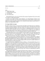
Figure 1.7:
Tricycle-drive configurations employing a steerable driven wheel and
two passive trailing wheels can derive heading information directly from a steering
angle encoder or indirectly from differential odometry [Everett, 1995].
1.3.2 Tricycle Drive
Tricycle-drive configurations (see Figure 1.7) employing a single driven front wheel and two passive
rear wheels (or vice versa) are fairly common in AGV applications because of their inherent
simplicity. For odometry instrumentation in the form of a steering-angle encoder, the dead-reckoning
solution is equivalent to that of an Ackerman-steered vehicle, where the steerable wheel replaces
the imaginary center wheel discussed in Section 1.3.3. Alternatively, if rear-axle differential
odometry is used to determine heading, the solution is identical to the differential-drive configuration
discussed in Section 1.3.1.
One problem associated with the tricycle-drive configuration is that the vehicle’s center of gravity
tends to move away from the front wheel when traversing up an incline, causing a loss of traction.
As in the case of Ackerman-steered designs, some surface damage and induced heading errors are
possible when actuating the steering while the platform is not moving.
1.3.3 Ackerman Steering
Used almost exclusively in the automotive industry, Ackerman steering is designed to ensure that
the inside front wheel is rotated to a slightly sharper angle than the outside wheel when turning,
thereby eliminating geometrically induced tire slippage. As seen in Figure 1.8, the extended axes for
the two front wheels intersect in a common point that lies on the extended axis of the rear axle. The
locus of points traced along the ground by the center of each tire is thus a set of concentric arcs
about this centerpoint of rotation P , and (ignoring for the moment any centrifugal accelerations) all
1

instantaneous velocity vectors will subsequently be tangential to these arcs. Such a steering geometry
is said to satisfy the Ackerman equation [Byrne et al., 1992]:
cot2
i
&cot2
o
'
d
l
cot2
SA
'
d
2l
% cot2
i
cot2
SA
' cot2
o
&
d
2l
.
Y
X
d
l
o
SA

i
P
2
P
1
22 Part I Sensors for Mobile Robot Positioning
(1.8)
(1.9)
(1.10)
Figure 1.8: In an Ackerman-steered vehicle, the extended axes for all wheels
intersect in a common point. (Adapted from [Byrne et al., 1992].)
where
2 = relative steering angle of the inner wheel
i
2 = relative steering angle of the outer wheel
o
l = longitudinal wheel separation
d = lateral wheel separation.
For the sake of convenience, the vehicle steering angle 2 can be thought of as the angle (relative
SA
to vehicle heading) associated with an imaginary center wheel located at a reference point P as
2
shown in the figure above. 2 can be expressed in terms of either the inside or outside steering
SA
angles (2 or 2 ) as follows [Byrne et al., 1992]:
i o
or, alternatively,
Ackerman steering provides a fairly accurate odometry solution while supporting the traction and
ground clearance needs of all-terrain operation. Ackerman steering is thus the method of choice for
outdoor autonomous vehicles. Associated drive implementations typically employ a gasoline or diesel

engine coupled to a manual or automatic transmission, with power applied to four wheels through
Rotation shaft
sprocket
Wheel
(Foot)
Steering chain
Drive chain
Upper torso
Steering
sprocket
Power
Steering
motor shaft
motor shaft
Drive
a.
b.
Chapter 1: Sensors for Dead Reckoning 23
Figure 1.9: A four-wheel synchro-drive configuration: a. Bottom view. b. Top view.
(Adapted from Holland [1983].)
a transfer case, a differential, and a series of universal joints. A representative example is seen in the
HMMWV-based prototype of the USMC Tele-Operated Vehicle (TOV) Program [Aviles et al.,
1990]. From a military perspective, the use of existing-inventory equipment of this type simplifies
some of the logistics problems associated with vehicle maintenance. In addition, reliability of the drive
components is high due to the inherited stability of a proven power train. (Significant interface
problems can be encountered, however, in retrofitting off-the-shelf vehicles intended for human
drivers to accommodate remote or computer control.)
1.3.4 Synchro Drive
An innovative configuration known as synchro drive features three or more wheels (Figure 1.9)
mechanically coupled in such a way that all rotate in the same direction at the same speed, and

similarly pivot in unison about their respective steering axes when executing a turn. This drive and
steering “synchronization” results in improved odometry accuracy through reduced slippage, since
all wheels generate equal and parallel force vectors at all times.
The required mechanical synchronization can be accomplished in a number of ways, the most
common being a chain, belt, or gear drive. Carnegie Mellon University has implemented an
electronically synchronized version on one of their Rover series robots, with dedicated drive motors
for each of the three wheels. Chain- and belt-drive configurations experience some degradation in
steering accuracy and alignment due to uneven distribution of slack, which varies as a function of
loading and direction of rotation. In addition, whenever chains (or timing belts) are tightened to
reduce such slack, the individual wheels must be realigned. These problems are eliminated with a
completely enclosed gear-drive approach. An enclosed gear train also significantly reduces noise as
well as particulate generation, the latter being very important in clean-room applications.
An example of a three-wheeled belt-drive implementation is seen in the Denning Sentry formerly
manufactured by Denning Mobile Robots, Woburn, MA [Kadonoff, 1986] and now by Denning
Branch Robotics International [DBIR]. Referring to Figure 1.9, drive torque is transferred down
through the three steering columns to polyurethane-filled rubber tires. The drive-motor output shaft
is mechanically coupled to each of the steering-column power shafts by a heavy-duty timing belt to
ensure synchronous operation. A second timing belt transfers the rotational output of the steering
motor to the three steering columns, allowing them to synchronously pivot throughout a full 360-
r
r'
B
Power shaft
90 Miter gear
A
A
B
'
r
)

r
24 Part I Sensors for Mobile Robot Positioning
Figure 1.10: Slip compensation during a turn is
accomplished through use of an offset foot assembly on
the three-wheeled K2A Navmaster robot. (Adapted from
[Holland, 1983].)
(1.11)
degree range [Everett, 1985]. The Sentry’s upper head assembly is mechanically coupled to the
steering mechanism in a manner similar to that illustrated in Figure 1.9, and thus always points in the
direction of forward travel. The three-point configuration ensures good stability and traction, while
the actively driven large-diameter wheels provide more than adequate obstacle climbing capability for
indoor scenarios. The disadvantages of this particular implementation include odometry errors
introduced by compliance in the drive belts as well as by reactionary frictional forces exerted by the
floor surface when turning in place.
To overcome these problems, the Cybermotion K2A Navmaster robot employs an enclosed gear-
drive configuration with the wheels offset from the steering axis as shown in Figure 1.10 and Figure
1.11. When a foot pivots during a turn, the attached wheel rotates in the appropriate direction to
minimize floor and tire wear, power consumption, and slippage. Note that for correct compensation,
the miter gear on the wheel axis must be on the opposite side of the power shaft gear from the wheel
as illustrated. The governing equation for minimal slippage is [Holland, 1983]
where
A = number of teeth on the power shaft gear
B = number of teeth on the wheel axle
gear
r’ = wheel offset from steering pivot axis
r = wheel radius.
One drawback of this approach is seen
in the decreased lateral stability that re-
sults when one wheel is turned in under
the vehicle. Cybermotion’s improved K3A

design solves this problem (with an even
smaller wheelbase) by incorporating a
dual-wheel arrangement on each foot
[Fisher et al., 1994]. The two wheels turn
in opposite directions in differential fash-
ion as the foot pivots during a turn, but
good stability is maintained in the forego-
ing example by the outward swing of the
additional wheel.
The odometry calculations for the
synchro drive are almost trivial; vehicle
heading is simply derived from the
steering-angle encoder, while displace-
ment in the direction of travel is given as
follows:
D
2 N
C
e
R
e
Chapter 1: Sensors for Dead Reckoning 25
(1.12)
Figure 1.11: The Denning
Sentry
(foreground) incorporates a three-point
synchro-drive
configuration with each wheel located directly below the pivot axis of the associated steering
column. In contrast, the Cybermotion
K2A

(background) has wheels that swivel around the
steering column. Both robots were extensively tested at the University of Michigan's Mobile
Robotics Lab. (Courtesy of The University of Michigan.)
where
D = vehicle displacement along path
N = measured counts of drive motor shaft encoder
C = encoder counts per complete wheel revolution
e
R = effective wheel radius.
e
1.3.5 Omnidirectional Drive
The odometry solution for most multi-degree-of-freedom (MDOF) configurations is done in similar
fashion to that for differential drive, with position and velocity data derived from the motor (or
wheel) shaft encoders. For the three-wheel example illustrated in Figure 1.12, the equations of
motion relating individual motor speeds to velocity components V and V in the reference frame of
xy
the vehicle are given by [Holland, 1983]:
a.
Top view
b.
R
Motor 2
of base
Motor 1
Forward
Motor 3
mdof01.ds4, mdof01.wmf, 5/19/94
26 Part I Sensors for Mobile Robot Positioning
Figure 1.12: a. Schematic of the wheel assembly used by the Veterans
Administration [La et al., 1981] on an omnidirectional wheelchair.

b. Top view of base showing relative orientation of components in
the three-wheel configuration. (Adapted from [Holland, 1983].)
Figure 1.13: A 4-degree-of-freedom
vehicle platform can travel in all
directions, including sideways and
diagonally. The difficulty lies in
coordinating all four motors so as to
avoid slippage.
V = T r = V + T R
1 1 x p
V = T r = -0.5V + 0.867V + T R (1.13)
2 2 x y p
V = T r = -0.5V - 0.867V + T R
3 3 x y p
where
V = tangential velocity of wheel number i
i
T = rotational speed of motor number i
i
T = rate of base rotation about pivot axis
p
T = effective wheel radius
r
T = effective wheel offset from pivot axis.
R
1.3.6 Multi-Degree-of-Freedom Vehicles
Multi-degree-of-freedom (MDOF) vehicles have multiple
drive and steer motors. Different designs are possible. For
example, HERMIES-III, a sophisticated platform designed
and built at the Oak Ridge National Laboratory [Pin et al.,

1989; Reister et al., 1991; Reister, 1991] has two powered
wheels that are also individually steered (see Figure 1.13).
With four independent motors, HERMIES-III is a 4-degree-
of-freedom vehicle.
MDOF configurations display exceptional maneuverability
in tight quarters in comparison to conventional 2-DOF
mobility systems, but have been found to be difficult to
control due to their overconstrained nature [Reister et al.,
1991; Killough and Pin, 1992; Pin and Killough, 1994;
Borenstein, 1995]. Resulting problems include increased
wheel slippage and thus reduced odometry accuracy.
Recently, Reister and Unseren [1992; 1993] introduced a
new control algorithm based on Force Control. The re-
searchers reported on a substantial reduction in wheel
Chapter 1: Sensors for Dead Reckoning 27
Figure 1.14: An 8-DOF platform with four wheels individually driven and steered.
This platform was designed and built by
Unique Mobility, Inc.
(Courtesy of
[UNIQUE].)
slippage for their two-wheel drive/two-wheel steer platform, resulting in a reported 20-fold
improvement of accuracy. However, the experiments on which these results were based avoided
simultaneous steering and driving of the two steerable drive wheels. In this way, the critical problem
of coordinating the control of all four motors simultaneously and during transients was completely
avoided.
Unique Mobility, Inc. built an 8-DOF vehicle for the U.S. Navy under an SBIR grant (see
Figure 1.14). In personal correspondence, engineers from that company mentioned to us difficulties
in controlling and coordinating all eight motors.
1.3.7 MDOF Vehicle with Compliant Linkage
To overcome the problems of control and the resulting excessive wheel slippage described above,

researchers at the University of Michigan designed the unique Multi-Degree-of-Freedom (MDOF)
vehicle shown in Figures 1.15 and 1.16 [Borenstein, 1992; 1993; 1994c; 1995]. This vehicle
comprises two differential-drive LabMate robots from [TRC]. The two LabMates, here referred to
as “trucks,” are connected by a compliant linkage and two rotary joints, for a total of three internal
degrees of freedom.
The purpose of the compliant linkage is to accommodate momentary controller errors without
transferring any mutual force reactions between the trucks, thereby eliminating the excessive wheel
slippage reported for other MDOF vehicles. Because it eliminates excessive wheel slippage, the
MDOF vehicle with compliant linkage is one to two orders of magnitude more accurate than other
MDOF vehicles, and as accurate as conventional, 2-DOF vehicles.
Truck A
Truck B
\book\clap30.ds4, clap30.w mf, 07/ 19/95
Drive
wheel
Castor
Drive
wheel
Drive
wheel
Drive
wheel
Castor
footprint
d
max
min
d
Track
28 Part I Sensors for Mobile Robot Positioning

Figure 1.15
: The compliant linkage is
instrumented with two absolute rotary
encoders and a linear encoder to
measure the relative orientations and
separation distance between the two
trucks.
Figure 1.16:
The University of Michigan's MDOF vehicle is a dual-
differential-drive multi-degree-of-freedom platform comprising two
TRC
LabMates
. These two "trucks” are coupled together with a
compliant linkage
, designed to accommodate momentary controller
errors that would cause excessive wheel slippage in other MDOF
vehicles. (Courtesy of The University of Michigan.)
Figure 1.17:
The effective point of contact for a skid-steer vehicle is
roughly constrained on either side by a rectangular zone of ambiguity
corresponding to the track footprint. As is implied by the concentric
circles, considerable slippage must occur in order for the vehicle to
turn [Everett, 1995].
1.3.8 Tracked Vehicles
Yet another drive configuration for
mobile robots uses tracks instead of
wheels. This very special imple-
mentation of a differential drive is
known as skid steering and is rou-
tinely implemented in track form

on bulldozers and armored vehi-
cles. Such skid-steer configurations
intentionally rely on track or wheel
slippage for normal operation (Fig-
ure 1.17), and as a consequence
provide rather poor dead-reckoning
information. For this reason, skid
steering is generally employed only
in tele-operated as opposed to au-
tonomous robotic applications, where the ability to surmount significant floor discontinuities is more
desirable than accurate odometry information. An example is seen in the track drives popular with
remote-controlled robots intended for explosive ordnance disposal. Figure 1.18 shows the Remotec
Andros V platform being converted to fully autonomous operation (see Sec. 5.3.1.2).
Chapter 1: Sensors for Dead Reckoning 29
Figure 1.18: A Remotec
Andros V
tracked vehicle is outfitted with computer control
at the University of Michigan. Tracked mobile platforms are commonly used in tele-
operated applications. However, because of the lack of odometry feedback they are
rarely (if at all) used in fully autonomous applications. (Courtesy of The University of
Michigan.)
Apparent Drift Calculation
(Reproduced with permission from [Sammarco, 1990].)
Apparent drift is a change in the output of the gyro-
scope as a result of the Earth's rotation. This change
in output is at a constant rate; however, this rate
depends on the location of the gyroscope on the Earth.
At the North Pole, a gyroscope encounters a rotation of
360 per 24-h period or 15 /h. The apparent drift will
vary as a sine function of the latitude as a directional

gyroscope moves southward. The direction of the
apparent drift will change once in the southern
hemisphere. The equations for Northern and Southern
Hemisphere apparent drift follow. Counterclockwise
(ccw) drifts are considered positive and clockwise (cw)
drifts are considered negative.
Northern Hemisphere: 15 /h [sin (latitude)] ccw.
Southern Hemisphere: 15 /h [sin (latitude,)] cw.
The apparent drift for Pittsburgh, PA (40.443 latitude) is
calculated as follows: 15 /h [sin (40.443)] = 9.73 /h
CCW or apparent drift = 0.162 /min. Therefore, a gyro-
scope reading of 52 at a time period of 1 minute would
be corrected for apparent drift where
corrected reading = 52 - (0.162 /min)(1 min) = 51.838 .
Small changes in latitude generally do not require
changes in the correction factor. For example, a 0.2
change in latitude (7 miles) gives an additional apparent
drift of only 0.00067 /min.
C
HAPTER
2
H
EADING
S
ENSORS
Heading sensors are of particular importance to mobile robot positioning because they can help
compensate for the foremost weakness of odometry: in an odometry-based positioning method, any
small momentary orientation error will cause a constantly growing lateral position error. For this
reason it would be of great benefit if orientation errors could be detected and corrected immediately.
In this chapter we discuss gyroscopes and compasses, the two most widely employed sensors for

determining the heading of a mobile robot (besides, of course, odometry). Gyroscopes can be
classified into two broad categories: (a) mechanical gyroscopes and (b) optical gyroscopes.

2.1 Mechanical Gyroscopes
The mechanical gyroscope, a well-known and reliable rotation sensor based on the inertial properties
of a rapidly spinning rotor, has been around since the early 1800s. The first known gyroscope was
built in 1810 by G.C. Bohnenberger of Germany. In 1852, the French physicist Leon Foucault
showed that a gyroscope could detect the rotation of the earth [Carter, 1966]. In the following
sections we discuss the principle of operation of various gyroscopes.
Anyone who has ever ridden a bicycle has experienced (perhaps unknowingly) an interesting
characteristic of the mechanical gyroscope known as gyroscopic precession. If the rider leans the
bike over to the left around its own horizontal axis, the front wheel responds by turning left around
the vertical axis. The effect is much more noticeable if the wheel is removed from the bike, and held
by both ends of its axle while rapidly spinning. If the person holding the wheel attempts to yaw it left
or right about the vertical axis, a surprisingly violent reaction will be felt as the axle instead twists
about the horizontal roll axis. This is due to the angular momentum associated with a spinning
flywheel, which displaces the applied force by 90 degrees in the direction of spin. The rate of
precession is proportional to the applied torque T [Fraden, 1993]:
Chapter 2: Heading Sensors 31
T = I (2.1)
where
T = applied input torque
I = rotational inertia of rotor
= rotor spin rate
= rate of precession.
Gyroscopic precession is a key factor involved in the concept of operation for the north-seeking
gyrocompass, as will be discussed later.
Friction in the support bearings, external influences, and small imbalances inherent in the
construction of the rotor cause even the best mechanical gyros to drift with time. Typical systems
employed in inertial navigation packages by the commercial airline industry may drift about 0.1

during a 6-hour flight [Martin, 1986].
2.1.1 Space-Stable Gyroscopes
The earth’s rotational velocity at any given point on the globe can be broken into two components:
one that acts around an imaginary vertical axis normal to the surface, and another that acts around
an imaginary horizontal axis tangent to the surface. These two components are known as the vertical
earth rate and the horizontal earth rate, respectively. At the North Pole, for example, the
component acting around the local vertical axis (vertical earth rate) would be precisely equal to the
rotation rate of the earth, or 15 /hr. The horizontal earth rate at the pole would be zero.
As the point of interest moves down a meridian toward the equator, the vertical earth rate at that
particular location decreases proportionally to a value of zero at the equator. Meanwhile, the
horizontal earth rate, (i.e., that component acting around a horizontal axis tangent to the earth’s
surface) increases from zero at the pole to a maximum value of 15 /hr at the equator.
There are two basic classes of rotational sensing gyros: 1) rate gyros, which provide a voltage or
frequency output signal proportional to the turning rate, and 2) rate integrating gyros, which indicate
the actual turn angle [Udd, 1991]. Unlike the magnetic compass, however, rate integrating gyros can
only measure relative as opposed to absolute angular position, and must be initially referenced to a
known orientation by some external means.
A typical gyroscope configuration is shown in Figure 2.1. The electrically driven rotor is
suspended in a pair of precision low-friction bearings at either end of the rotor axle. The rotor
bearings are in turn supported by a circular ring, known as the inner gimbal ring; this inner gimbal
ring pivots on a second set of bearings that attach it to the outer gimbal ring. This pivoting action
of the inner gimbal defines the horizontal axis of the gyro, which is perpendicular to the spin axis of
the rotor as shown in Figure 2.1. The outer gimbal ring is attached to the instrument frame by a third
set of bearings that define the vertical axis of the gyro. The vertical axis is perpendicular to both the
horizontal axis and the spin axis.
Notice that if this configuration is oriented such that the spin axis points east-west, the horizontal
axis is aligned with the north-south meridian. Since the gyro is space-stable (i.e., fixed in the inertial
reference frame), the horizontal axis thus reads the horizontal earth rate component of the planet’s
rotation, while the vertical axis reads the vertical earth rate component. If the spin axis is rotated 90
degrees to a north-south alignment, the earth’s rotation does not affect the gyro’s horizontal axis,

since that axis is now orthogonal to the horizontal earth rate component.
Outer gimbal
Wheel bearing
Wheel
Inner gimbal
Outer pivot
Inner pivot
32 Part I Sensors for Mobile Robot Positioning
Figure 2.1:
Typical two-axis mechanical gyroscope configuration [Everett, 1995].
2.1.2 Gyrocompasses
The gyrocompass is a special configuration of the rate integrating gyroscope, employing a gravity
reference to implement a north-seeking function that can be used as a true-north navigation
reference. This phenomenon, first demonstrated in the early 1800s by Leon Foucault, was patented
in Germany by Herman Anschutz-Kaempfe in 1903, and in the U.S. by Elmer Sperry in 1908 [Carter,
1966]. The U.S. and German navies had both introduced gyrocompasses into their fleets by 1911
[Martin, 1986].
The north-seeking capability of the gyrocompass is directly tied to the horizontal earth rate
component measured by the horizontal axis. As mentioned earlier, when the gyro spin axis is
oriented in a north-south direction, it is insensitive to the earth's rotation, and no tilting occurs. From
this it follows that if tilting is observed, the spin axis is no longer aligned with the meridian. The
direction and magnitude of the measured tilt are directly related to the direction and magnitude of
the misalignment between the spin axis and true north.
2.1.3 Commercially Available Mechanical Gyroscopes
Numerous mechanical gyroscopes are available on the market. Typically, these precision machined
gyros can cost between $10,000 and $100,000. Lower cost mechanical gyros are usually of lesser
quality in terms of drift rate and accuracy. Mechanical gyroscopes are rapidly being replaced by
modern high-precision — and recently — low-cost fiber-optic gyroscopes. For this reason we will
discuss only a few low-cost mechanical gyros, specifically those that may appeal to mobile robotics
hobbyists.

Chapter 2: Heading Sensors 33
Figure 2.2: The Futaba FP-G154 miniature mechanical
gyroscope for radio-controlled helicopters. The unit costs
less than $150 and weighs only 102 g (3.6 oz).
Figure 2.3: The Gyration
GyroEngine
compares in size
favorably with a roll of 35 mm film (courtesy Gyration, Inc.).
2.1.3.1 Futaba Model Helicopter Gyro
The Futaba FP-G154 [FUTABA] is a low-
cost low-accuracy mechanical rate gyro
designed for use in radio-controlled model
helicopters and model airplanes. The Futaba
FP-G154 costs less than $150 and is avail-
able at hobby stores, for example [TOWER].
The unit comprises of the mechanical gyro-
scope (shown in Figure 2.2 with the cover
removed) and a small control amplifier.
Designed for weight-sensitive model helicop-
ters, the system weighs only 102 grams
(3.6 oz). Motor and amplifier run off a 5 V
DC supply and consume only 120 mA.
However, sensitivity and accuracy are orders
of magnitude lower than “professional”
mechanical gyroscopes. The drift of radio-control type gyroscopes is on the order of tens of degrees
per minute.
2.1.3.2 Gyration, Inc.
The GyroEngine made by Gyration, Inc.
[GYRATION], Saratoga, CA, is a low-cost
mechanical gyroscope that measures

changes in rotation around two independ-
ent axes. One of the original applications
for which the GyroEngine was designed is
the GyroPoint, a three-dimensional point-
ing device for manipulating a cursor in
three-dimensional computer graphics. The
GyroEngine model GE9300-C has a typi-
cal drift rate of about 9 /min. It weighs
only 40 grams (1.5 oz) and compares in
size with that of a roll of 35 millimeter film
(see Figure 2.3). The sensor can be pow-
ered with 5 to 15 VDC and draws only 65
to 85 mA during operation. The open collector outputs can be readily interfaced with digital circuits.
A single GyroEngine unit costs $295.
2.2 Piezoelectric Gyroscopes
Piezoelectric vibrating gyroscopes use Coriolis forces to measure rate of rotation. in one typical
design three piezoelectric transducers are mounted on the three sides of a triangular prism. If one
of the transducers is excited at the transducer's resonance frequency (in the Gyrostar it is 8 kHz),
34 Part I Sensors for Mobile Robot Positioning
Figure 2.4: The Murata
Gyrostar
ENV-05H is a piezoelectric
vibrating gyroscope. (Courtesy of [Murata]).
the vibrations are picked up by the two other transducers at equal intensity. When the prism is
rotated around its longitudinal axis, the resulting Coriolis force will cause a slight difference in the
intensity of vibration of the two measuring transducers. The resulting analog voltage difference is
an output that varies linearly with the measured rate of rotation.
One popular piezoelectric vibrating gyroscope is the ENV-05 Gyrostar from [MURATA], shown
in Fig. 2.4. The Gyrostar is small, lightweight, and inexpensive: the model ENV-05H measures
47×40×22 mm (1.9×1.6×0.9 inches), weighs 42 grams (1.5 oz) and costs $300. The drift rate, as

quoted by the manufacturer, is very poor: 9 /s. However, we believe that this number is the worst
case value, representative for extreme temperature changes in the working environment of the
sensor. When we tested a Gyrostar Model ENV-05H at the University of Michigan, we measured
drift rates under typical room temperatures of 0.05 /s to 0.25 /s, which equates to 3 to 15 /min (see
[Borenstein and Feng, 1996]). Similar drift rates were reported by Barshan and Durrant-Whyte
[1995], who tested an earlier model: the Gyrostar ENV-05S (see Section 5.4.2.1 for more details on
this work). The scale factor, a measure for the useful sensitivity of the sensor, is quoted by the
manufacturer as 22.2 mV/deg/sec.
2.3 Optical Gyroscopes
Optical rotation sensors have now been under development as replacements for mechanical gyros
for over three decades. With little or no moving parts, such devices are virtually maintenance free
and display no gravitational sensitivities, eliminating the need for gimbals. Fueled by a large
EM field pattern
is stationary in
inertial frame
Observer moves
around ring
with rotation
Lossless
cylindrical
Nodes
mirror
Chapter 2: Heading Sensors 35
Figure 2.5: Standing wave created by counter-propagating light beams in
an idealized ring-laser gyro. (Adapted from [Schulz-DuBois, 1966].)
market in the automotive industry, highly linear fiber-optic versions are now evolving that have wide
dynamic range and very low projected costs.
The principle of operation of the optical gyroscope, first discussed by Sagnac [1913], is
conceptually very simple, although several significant engineering challenges had to be overcome
before practical application was possible. In fact, it was not until the demonstration of the helium-

neon laser at Bell Labs in 1960 that Sagnac’s discovery took on any serious implications; the first
operational ring-laser gyro was developed by Warren Macek of Sperry Corporation just two years
later [Martin, 1986]. Navigation quality ring-laser gyroscopes began routine service in inertial
navigation systems for the Boeing 757 and 767 in the early 1980s, and over half a million fiber-optic
navigation systems have been installed in Japanese automobiles since 1987 [Reunert, 1993]. Many
technological improvements since Macek’s first prototype make the optical rate gyro a potentially
significant influence on mobile robot navigation in the future.
The basic device consists of two laser beams traveling in opposite directions (i.e., counter
propagating) around a closed-loop path. The constructive and destructive interference patterns
formed by splitting off and mixing parts of the two beams can be used to determine the rate and
direction of rotation of the device itself.
Schulz-DuBois [1966] idealized the ring laser as a hollow doughnut-shaped mirror in which light
follows a closed circular path. Assuming an ideal 100-percent reflective mirror surface, the optical
energy inside the cavity is theoretically unaffected by any rotation of the mirror itself. The counter-
propagating light beams mutually reinforce each other to create a stationary standing wave of
intensity peaks and nulls as depicted in Figure 2.5, regardless of whether the gyro is rotating [Martin,
1986].
A simplistic visualization based on the Schulz-DuBois idealization is perhaps helpful at this point in
understanding the fundamental concept of operation before more detailed treatment of the subject
is presented. The light and dark fringes of the nodes are analogous to the reflective stripes or slotted
holes in the rotating disk of an incremental optical encoder, and can be theoretically counted in similar
fashion by a light detector mounted on the cavity wall. (In this analogy, however, the standing-wave
“disk” is fixed in the inertial reference frame, while the normally stationary detector revolves around
it.) With each full rotation of the mirrored doughnut, the detector would see a number of node peaks
equal to twice the optical path length of the beams divided by the wavelength of the light.
L
4 r
2
c
36 Part I Sensors for Mobile Robot Positioning

(2.2)
Obviously, there is no practical way to implement this theoretical arrangement, since a perfect
mirror cannot be realized in practice. Furthermore, the introduction of light energy into the cavity
(as well as the need to observe and count the nodes on the standing wave) would interfere with the
mirror's performance, should such an ideal capability even exist. However, many practical
embodiments of optical rotation sensors have been developed for use as rate gyros in navigation
applications. Five general configurations will be discussed in the following subsections:
Active optical resonators (2.3.1).
Passive optical resonators (2.3.2).
Open-loop fiber-optic interferometers (analog) (2.3.3).
Closed-loop fiber-optic interferometers (digital) (2.3.4).
Fiber-optic resonators (2.3.5).
Aronowitz [1971], Menegozzi and Lamb [1973], Chow et al. [1985], Wilkinson [1987], and Udd
[1991] provide in-depth discussions of the theory of the ring-laser gyro and its fiber-optic
derivatives. A comprehensive treatment of the technologies and an extensive bibliography of
preceding works is presented by Ezekial and Arditty [1982] in the proceedings of the First
International Conference on Fiber-Optic Rotation Sensors held at MIT in November, 1981. An
excellent treatment of the salient features, advantages, and disadvantages of ring laser gyros versus
fiber optic gyros is presented by Udd [1985, 1991].
2.3.1 Active Ring Laser Gyros
The active optical resonator configuration, more commonly known as the ring laser gyro, solves the
problem of introducing light into the doughnut by filling the cavity itself with an active lazing
medium, typically helium-neon. There are actually two beams generated by the laser, which travel
around the ring in opposite directions. If the gyro cavity is caused to physically rotate in the
counterclockwise direction, the counterclockwise propagating beam will be forced to traverse a
slightly longer path than under stationary conditions. Similarly, the clockwise propagating beam will
see its closed-loop path shortened by an identical amount. This phenomenon, known as the Sagnac
effect, in essence changes the length of the resonant cavity. The magnitude of this change is given
by the following equation [Chow et al., 1985]:
where

L = change in path length
r = radius of the circular beam path
= angular velocity of rotation
c = speed of light.
Note that the change in path length is directly proportional to the rotation rate of the cavity.
Thus, to measure gyro rotation, some convenient means must be established to measure the induced
change in the optical path length.
This requirement to measure the difference in path lengths is where the invention of the laser in
the early 1960s provided the needed technological breakthrough that allowed Sagnac’s observations
to be put to practical use. For lazing to occur in the resonant cavity, the round-trip beam path must
f
2fr
c
2r
f
4A
P
Chapter 2: Heading Sensors 37
(2.3)
(2.4)
be precisely equal in length to an integral number of wavelengths at the resonant frequency. This
means the wavelengths (and therefore the frequencies) of the two counter- propagating beams must
change, as only oscillations with wavelengths satisfying the resonance condition can be sustained
in the cavity. The frequency difference between the two beams is given by [Chow et al., 1985]:
where
f = frequency difference
r = radius of circular beam path
= angular velocity of rotation
= wavelength.
In practice, a doughnut-shaped ring cavity would be hard to realize. For an arbitrary cavity

geometry, the expression becomes [Chow et al., 1985]:
where
f = frequency difference
A = area enclosed by the closed-loop beam path
= angular velocity of rotation
P = perimeter of the beam path
= wavelength.
For single-axis gyros, the ring is generally formed by aligning three highly reflective mirrors to
create a closed-loop triangular path as shown in Figure 2.6. (Some systems, such as Macek’s early
prototype, employ four mirrors to create a square path.) The mirrors are usually mounted to a
monolithic glass-ceramic block with machined ports for the cavity bores and electrodes. Most
modern three-axis units employ a square block cube with a total of six mirrors, each mounted to the
center of a block face as shown in Figure 2.6. The most stable systems employ linearly polarized light
and minimize circularly polarized components to avoid magnetic sensitivities [Martin, 1986].
The approximate quantum noise limit for the ring-laser gyro is due to spontaneous emission in the
gain medium [Ezekiel and Arditty, 1982]. Yet, the ring-laser gyro represents the “best-case” scenario
of the five general gyro configurations outlined above. For this reason the active ring-laser gyro
offers the highest sensitivity and is perhaps the most accurate implementation to date.
The fundamental disadvantage associated with the active ring laser is a problem called frequency
lock-in, which occurs at low rotation rates when the counter-propagating beams “lock” together in
frequency [Chao et al., 1984]. This lock-in is attributed to the influence of a very small amount of
backscatter from the mirror surfaces, and results in a deadband region (below a certain threshold of
rotational velocity) for which there is no output signal. Above the lock-in threshold, output
approaches the ideal linear response curve in a parabolic fashion.
The most obvious approach to solving the lock-in problem is to improve the quality of the mirrors
to reduce the resulting backscatter. Again, however, perfect mirrors do not exist, and some finite
B
CD
A
38 Part I Sensors for Mobile Robot Positioning

Figure 2.6: Six-mirror configuration of three-axis ring-laser
gyro. (Adapted from [Koper, 1987].)
amount of backscatter will always be present. Martin [1986] reports a representative value as 10
-12
of the power of the main beam; enough to induce frequency lock-in for rotational rates of several
hundred degrees per hour in a typical gyro with a 20-centimeter (8-in) perimeter.
An additional technique for reducing lock-in is to incorporate some type of biasing scheme to shift
the operating point away from the deadband zone. Mechanical dithering is the least elegant but most
common biasing means, introducing the obvious disadvantages of increased system complexity and
reduced mean time between failures due to the moving parts. The entire gyro assembly is rotated
back and forth about the sensing axis in an oscillatory fashion. State-of-the-art dithered active ring
laser gyros have a scale factor linearity that far surpasses the best mechanical gyros.
Dithered biasing, unfortunately, is too slow for high-performance systems (i.e., flight control),
resulting in oscillatory instabilities [Martin, 1986]. Furthermore, mechanical dithering can introduce
crosstalk between axes on a multi-axis system, although some unibody three-axis gyros employ a
common dither axis to eliminate this possibility [Martin, 1986].
Buholz and Chodorow [1967], Chesnoy [1989], and Christian and Rosker [1991] discuss the use
of extremely short duration laser pulses (typically 1/15 of the resonator perimeter in length) to
reduce the effects of frequency lock-in at low rotation rates. The basic idea is to reduce the cross-
coupling between the two counter-propagating beams by limiting the regions in the cavity where the
two pulses overlap. Wax and Chodorow [1972] report an improvement in performance of two orders
of magnitude through the use of intracavity phase modulation. Other techniques based on non-linear
optics have been proposed, including an approach by Litton that applies an external magnetic field
to the cavity to create a directionally dependent phase shift for biasing [Martin, 1986]. Yet another
solution to the lock-in problem is to remove the lazing medium from the ring altogether, effectively
forming what is known as a passive ring resonator.
Light source
Detector
Partially
transmissive

mirror
Highly
reflective
mirror
n '
c
c
m
Chapter 2: Heading Sensors 39
Figure 2.7: Passive ring resonator gyro with laser source
external to the ring cavity. (Adapted from [Udd, 1991].)
(2.5)
2.3.2 Passive Ring Resonator Gyros
The passive ring resonator gyro makes use of a laser source external to the ring cavity
(Figure 2.7), and thus avoids the frequency lock-in problem which arises when the gain medium is
internal to the cavity itself. The passive configuration also eliminates problems arising from changes
in the optical path length within the interferometer due to variations in the index of refraction of the
gain medium [Chow et al., 1985]. The theoretical quantum noise limit is determined by photon shot
noise and is slightly higher (i.e., worse) than the theoretical limit seen for the active ring-laser gyro
[Ezekiel and Arditty, 1982].
The fact that these devices use mirrored resonators patterned after their active ring predecessors
means that their packaging is inherently bulky. However, fiber-optic technology now offers a low
volume alternative. The fiber-optic derivatives also allow longer length multi-turn resonators, for
increased sensitivity in smaller, rugged, and less expensive packages. As a consequence, the Resonant
Fiber-Optic Gyro (RFOG), to be discussed in Section 2.1.2.5, has emerged as the most popular of
the resonator configurations [Sanders, 1992].
2.3.3 Open-Loop Interferometric Fiber Optic Gyros
The concurrent development of optical fiber technology, spurred mainly by the communications
industry, presented a potential low-cost alternative to the high-tolerance machining and clean-room
assembly required for ring-laser gyros. The glass fiber in essence forms an internally reflective

waveguide for optical energy, along the lines of a small-diameter linear implementation of the
doughnut-shaped mirror cavity conceptualized by Schulz-DuBois [1966].
Recall the refractive index n relates the speed of light in a particular medium to the speed of light
in a vacuum as follows:
axis
n
co
n
cl
Waveguide
NA ' sin2
c
' n
2
co
&n
2
cl
2
1
Numerical aperture
Waveguide
axis
40 Part I Sensors for Mobile Robot Positioning
Figure 2.8: Step-index multi-mode fiber. (Adapted from
[Nolan et al., 1991].)
(2.6)
Figure 2.9: Entry angles of incoming rays 1 and 2
determine propagation paths in fiber core. (Adapted from
[Nolan et al., 1991].)

where
n = refractive index of medium
c = speed of light in a vacuum
c = speed of light in medium.
m
Step-index multi-mode fiber (Figure 2.8) is made up of a core region of glass with index of
refraction n , surrounded by a protective cladding with a lower index of refraction n [Nolan and
co cl
Blaszyk, 1991]. The lower refractive index in the cladding is necessary to ensure total internal
reflection of the light propagating through the core region. The terminology step index refers to this
“stepped” discontinuity in the refractive index that occurs at the core-cladding interface.
Referring now to Figure 2.8, as long as the entry angle (with respect to the waveguide axis) of an
incoming ray is less than a certain critical angle 2 , the ray will be guided down the fiber, virtually
c
without loss. The numerical aperture of the fiber quantifies this parameter of acceptance (the light-
collecting ability of the fiber) and is defined as follows [Nolan and Blaszyk, 1991]:
where
NA = numerical aperture of the fiber
2 = critical angle of acceptance
c
n = index of refraction of glass core
co
n = index of refraction of cladding.
cl
As illustrated in Figure 2.9, a number of rays following different-length paths can simultaneously
propagate down the fiber, as long as their respective entry angles are less than the critical angle of
acceptance 2 . Multiple-path propagation of this nature occurs where the core diameter is much larger
c
than the wavelength of the guided energy, giving rise to the term multi-mode fiber. Such multi-mode
operation is clearly undesirable in gyro applications, where the objective is to eliminate all non-

reciprocal conditions other than that imposed by the Sagnac effect itself. As the diameter of the core
is reduced to approach the operating wavelength, a cutoff condition is reached where just a single
mode is allowed to propagate, con-
strained to travel only along the wave-
guide axis [Nolan and Blaszyk, 1991].
Light can randomly change polariza
tion states as it propagates through stan-
dard single-mode fiber. The use of special
polarization-maintaining fiber, such as
PRSM Corning, maintains the original
polarization state of the light along the
path of travel [Reunert, 1993]. This is
important, since light of different polariza-
tion states travels through an optical fiber
at different speeds.