Ebook Ecotoxicology – A comprehensive treatment: Part 2

of
24 Application
Multimetric and

Multivariate Approaches
in Community
Ecotoxicology

The most distinct and beautiful statement of any truth must take at last the mathematical form.
(Henry David Thoreau, in Walls 1999)

24.1 INTRODUCTION
Methods to assess the effects of contaminants and other anthropogenic stressors on communities
range from computationally simple indices such as species richness to complex, computer-dependent
algorithms such as multivariate analyses. The simplest community indices use species presence/absence or abundance data to show how individuals in the community are distributed among
species. The advantages of these indices are their intuitive meaning and their ability to reduce complex
data to a single number. Only slightly more involved but retaining more information, species abundance curves described in Chapter 22 characterize the distribution of individuals among the species
by fitting abundance data to specified distributions. Estimated distributional parameters from species
abundance models provide a parsimonious description of the community. Slightly more involved
composite measures require additional knowledge about community qualities (e.g., the trophic status
of a species) to produce indices developed specifically to gauge diminished community integrity due
to anthropogenic stressors. Currently, the most popular of these composite indices is Karr’s (1981)
index of biological integrity (IBI). These composite indices require more ecological knowledge of
the community than measures of species richness or species abundance models but have the advantage of being focused primarily on human effects on communities or species assemblages. More
convenient, but perhaps applying less ecology than warranted, distributions of individual species
effect metrics (e.g., distributions of 96-h LC50 values) are used to predict “safe concentrations” that
presumably protect all but a specified, low percentage of the species making up the community.
Even more computationally intense methods, such as multivariate analyses, aim to reduce the number of data dimensions to an interpretable low number, and to quantify similarities or differences
among sampling units. These last methods tend to generate interpretive parsimony at the expense
of methodological simplicity and straightforward terminology; therefore, considerable caution is
needed to avoid errors during their application. However, the value of these methods in identifying

clear explanations from complex data sets makes worthwhile any effort spent wading through obtuse
computer manuals or dealing with the associated jargon.
Jargon, not argument, is your best ally in keeping him from the Church.
(Lewis 1942)
473

Clements: “3357_c024” — 2007/11/9 — 18:34 — page 473 — #1


474

Ecotoxicology: A Comprehensive Treatment

24.1.1 COMPARISON OF MULTIMETRIC AND MULTIVARIATE
APPROACHES
Multimetric and multivariate approaches are applied to community data with the intent of rendering the associated complex array of information to a more parsimonious form. Because ecological
assessments of biological integrity generally require analysis of numerous biotic and abiotic variables, sophisticated statistical approaches are often necessary to examine the complex relationships
between species assemblages and multiple environmental factors. Multivariate approaches reduce
complex, multidimensional data to two or three dimensions, thus allowing researchers to identify
key environmental variables responsible for patterns of species abundance. In contrast, multimetric
indices integrate a diverse suite of measures, often across several levels of biological organization,
to assess biological integrity. It is appropriate to consider these two approaches together because the
community data necessary to calculate a multimetric index or to conduct multivariate analyses are
often the same (e.g., abundance, richness, and composition).
In their comparison of multivariate and multimetric approaches, Reynoldson et al. (1997) concluded that multivariate approaches provided greater accuracy and precision for assessing reference
conditions in streams. Terlizzi et al. (2005) showed that univariate measures of molluscan community
structure (species richness) showed little response to contamination whereas multivariate analyses
identified significant differences between reference and polluted sites. Thomas and Hall (2006) compared the ability of individual metrics, multivariate approaches, and multimetric indices to identify
impairment in periphyton, macroinvertebrate, and fish communities. Although some individual metrics were associated with large-scale habitat gradients, multivariate approaches were most useful
for identifying spatial and temporal differences in each community. In a comprehensive analysis of

community indices and multivariate approaches, Kilgour et al. (2004) compared the relative sensitivity of seven benthic community metrics and three multivariate indices to contamination associated
with mines, pulp and paper mills, and urbanization. Multivariate approaches identified significant differences associated with each of the perturbations and greater effect sizes compared to the
community metrics. Although the examples described above seem to highlight the greater discriminatory ability of multivariate approaches, the usefulness of univariate and multivariate techniques
for distinguishing between reference and contaminated sites will likely vary with the spatial scale
of an investigation (Quintino et al. 2006). Despite their growing popularity in Canada and Europe,
multivariate approaches have received considerably less attention in the United States (Resh et al.
1995). Multivariate analyses have been criticized because of their inherent statistical complexity
and because results are often difficult to interpret (Fore et al. 1996, Gerritsen 1995). The complex graphical representations of multivariate results are often of limited value to non-ecologists
and managers. Although strict reliance on complex statistical algorithms may obscure important
biological results, we believe that multivariate approaches are an essential set of tools for biological assessments of water quality. Because community–environment relationships are inherently
multidimensional, approaches such as multivariate analyses that consider interactions among predictor variables and their effects on multiple response variables are necessary. New approaches,
such as the application of principal response curves (Pardal et al. 2004), quantify multivariate
community responses to contaminants in ways that are more accessible to managers and policymakers. We agree with the recommendations of Reynoldson et al. (1997) that multivariate and
multimetric approaches are complementary and should be used in conjunction. For example, the
variables used in multivariate analyses such as principal components could include species richness, abundance of sensitive groups, or other measures typically included in a multimetric index.
Griffith et al. (2003) used this approach in their evaluation of the relationship between macroinvertebrate assemblages and environmental gradients. Multivariate statistical analysis (redundancy
analysis) using metrics derived from an index of biotic integrity provided complementary results to canonical correspondence analysis based on macroinvertebrate abundance. Alternatively,

Clements: “3357_c024” — 2007/11/9 — 18:34 — page 474 — #2


Application of Multimetric and Multivariate Approaches in Community Ecotoxicology

475

a multimetric index similar to Karr’s IBI could be developed using results of multivariate analyses. Loading coefficients from canonical discriminant analyses, principal component analyses
(PCA), and other multivariate procedures identify variables that are most important for separation
of groups (generally locations, sampling stations). Variables shown to be responsible for separation of reference and impacted stations could be combined in a multimetric index. Integration of
multivariate and multimetric approaches may be necessary to detect perturbations when relatively
weak relationships between stressors and community structure exist (Chenery and Mudge 2005).

Finally, we note that our enthusiasm for multimetric and multivariate approaches in communitylevel bioassessment is not shared by all researchers. Weiss and Reice (2005) remind us that neither of
these approaches provides causal linkages between stressors and community-level responses. These
researchers advocate an alternative approach in which effects of stressors on individual taxa with
known species-level tolerances are employed to develop an overall assessment of community-level
impact.

24.2 MULTIMETRIC INDICES
A principal objective of the 1972 Federal Water Pollution Control Act and its 1977 and 1987 amendments
is to restore and maintain the biological integrity of the nation’s waters.
(Miller et al. 1988)

One of the most significant advances in the field of biological assessments over the past 20 years
was the development and application of multimetric approaches for measuring ecological integrity.
Because no single measure of impairment will respond to all classes of contaminants, and because
some individual metrics may show unexpected changes (e.g., increased species richness at polluted
sites), multimetric indices are an effective tool for measuring effects of stressors (Fausch et al. 1990,
Karr 1981, Kerans and Karr 1994, Plafkin et al. 1989). The individual metrics in a multimetric index
reflect different characteristics of life history, community structure, and functional organization. In
general, as the number of metrics increases (up to some reasonable number), the ability to separate
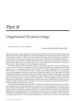
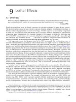
contaminant effects from natural variation increases (Karr 1993) (Figure 24.1). In addition, because

Ecological attribute

One metric

Two metrics

Threshold value

Level of stressor

Level of stressor

FIGURE 24.1 Hypothetical relationships between stressor levels and ecological attributes characterized using
one or two metrics. The threshold value of the ecological attribute is defined as the response that is considered
to be biologically significant. For example, a researcher may conclude that a 20% reduction in abundance of
a sensitive species is a biologically significant response. The responses of the individual metrics are represented
as clouds of points and the level of the stressor known to affect the ecological attribute is represented by the
black bar. Note that addition of a second metric provides a more refined measure of the stressor level that causes
a biologically significant response. (Modified from Figure 1 in Karr (1993).)

Clements: “3357_c024” — 2007/11/9 — 18:34 — page 475 — #3


476

Ecotoxicology: A Comprehensive Treatment

individual metrics respond differently to different classes of contaminants, multimetric approaches
are useful for assessing a diverse suite of stressors and measuring impacts in systems receiving
multiple stressors. The individual metrics included in a multimetric index may vary among perturbations, but should reflect important structural and functional characteristics of the system. In general,
deviation of individual metrics from expected values at reference sites is estimated and a final value
that includes the sum of all individual metrics is calculated.
Karr’s (1981) IBI is the most widely used multimetric index for assessing the health of aquatic
communities. The IBI was developed in response to the federally legislated mandate to “restore and
maintain the chemical, physical, and biological integrity” of U.S. waters (Clean Water Act 1977,
PL 95-217, also 1987 PL 100-4). Originally employed in Midwestern streams in the United States,
the IBI is based on 12 attributes of fish assemblages in three general categories: species richness
and composition, trophic composition, and fish abundance and condition. The individual metrics are
assigned scores (1, 3, 5) based on their similarity to expected values in undisturbed or least impacted

streams. Expected values for the individual metrics are obtained by sampling a large number of
known reference sites in a region. Alternatively, expected values can be derived from surveys of
reference and impacted sites and using the “best” values from these samples (Simon and Lyons
1995). Because expected values for species richness and total abundance vary with stream size,
these metrics must be adjusted to reflect watershed area and other regional conditions. The scores
of the 12 metrics are summed to yield a total IBI score for a site (which ranges from 12 to 60), with
larger values indicating healthy fish assemblages. The IBI is sensitive to a diverse array of physical
and chemical stressors, including industrial and municipal effluents, agricultural inputs, habitat loss,
and introduction of exotic species.
The IBI works especially well for characterizing fish communities because environmental
requirements and historic distributions of this group are well known. This greatly facilitates establishment of expected values for individual metrics. The structural and functional metrics included in
the IBI are biologically relevant, and each individual metric responds to known gradients of degradation (Fausch et al. 1990). The general approach outlined in the IBI has been modified for other
ecosystems (e.g., lakes and estuaries) and applied to other taxonomic groups (e.g., benthic macroinvertebrates and diatoms). Although the specific metrics vary among these applications, comparison
of measured values to expected values and integration of a suite of metrics into a single index
are consistent among approaches. A multimetric index for benthic macroinvertebrate communities
was used to distinguish polluted from reference sites in rivers of the Tennessee Valley (Kerans and
Karr 1994). The benthic IBI (B-IBI) was found to be highly effective because benthic macroinvertebrates generally respond to chemical and physical degradation in a predictable fashion. The
IBI now enjoys such popularity that the term, IBI, has come to be applied to any new composite
or multimetric index.
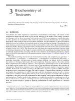
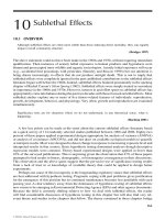
Calculating multimetric indices involves comparing individual metrics measured at an impacted
site to the expected values for the region (Figure 24.2a). As described above, because some
metrics (e.g., species richness) are greatly influenced by stream order and watershed area, these
expected values must be adjusted to reflect natural variation (Figure 24.2b). Assuming that
community responses to other landscape variables are predictable, a logical extension of this
approach is to create models to account for natural variation across broad geographical areas.
Bailey et al. (1998) found that simple geographic characteristics (distance from source, catchment area, elevation) and year sampled accounted for greater than 50% of the variation among
reference sites. The performance of several bioassessment metrics was significantly improved
when a predictive model that included this geographic variation was employed to identify
impacted sites. The conventional approach of comparing metric values at impacted sites with
expected values at reference sites has now advanced to the point where we can characterize habitat variation within subregions using more sophisticated multivariate statistics (Figure 24.2c).

The application of multivariate techniques for assessing reference conditions is described
below.

Clements: “3357_c024” — 2007/11/9 — 18:34 — page 476 — #4


Application of Multimetric and Multivariate Approaches in Community Ecotoxicology

(a)

477

(b)
Range of expected metric
values at reference sites
Expected metric value

Metric value

Test
site

Metric 1

al
erv

%

95

c

en

fid

n
Co

nt
ei

Test
site 2
Test
site 1

Metric 2

Habitat gradient

Multivariate axis 2

(c)
95% Confidence
ellipsoids
Test
site 1

Test
site 3

Test
site 2
Multivariate axis 1

FIGURE 24.2 Multimetric and multivariate approaches for comparing test sites to expected values at reference
sites. (a) Two metric values at a test site (indicated by solid circles) are compared to expected values. Values
are within the expected range for metric 1, but below the range of expected values for metric 2. (b) Metric
values are adjusted to reflect expected changes in habitat characteristics along a gradient. Although the metric
value at test site 2 is greater than at test site 1, it is less than the expected value and would indicate impact.
(c) Multivariate analysis of expected metric values based on regional differences in habitat characteristics. Test
sites 1 and 2 are within the expected values whereas test site 3 falls outside the 95% confidence ellipsoid.

24.2.1 MULTIMETRIC APPROACHES FOR TERRESTRIAL
COMMUNITIES
Although multimetric indices such as the IBI have been limited primarily to aquatic ecosystems,
the general approach could be modified for terrestrial communities. Because of their sensitivity
and rapid response to environmental stressors, terrestrial arthropods would be especially useful for
assessing biological integrity (Kremen et al. 1993). Nelson and Epstein (1998) investigated the
responses of lepidopterans to habitat modifications and concluded that butterfly communities integrate important structural and functional characteristics of terrestrial ecosystems. Kremen (1992)
evaluated the indicator properties of butterfly communities and reported that this group was quite
responsive to anthropogenic disturbance. Bird communities also offer opportunities for development
of integrated measures of ecological integrity. The abundance, distribution, and habitat requirements
of birds are generally well known, especially in North America. National monitoring programs,
such as the Christmas Bird Counts conducted by the Audubon Society and Breeding Bird Surveys, have provided spatially extensive, long-term data on bird assemblages. Finally, responses
of bird populations to some environmental stressors, especially pesticides and habitat alterations,
have been well documented. However, given the logistical difficulties of sampling bird communities, developing a suite of ecologically relevant indicators for this group will be a challenge. In

Clements: “3357_c024” — 2007/11/9 — 18:34 — page 477 — #5


Ecotoxicology: A Comprehensive Treatment

478

Species richness of butterflies

16
14
12
10
8
6
4
2
5

10

15

20

25

30

Species richness of birds

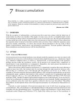
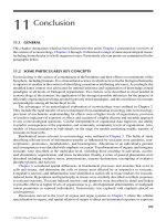
FIGURE 24.3 The relationship between species richness of birds and butterflies at 6 sites along a gradient of
urban development. Obtaining quantitative data for certain taxonomic groups, such as birds and small mammals
is often expensive and logistically challenging. The close relationship between these measures suggests that
butterflies, which are relatively easy to monitor, can be used as a surrogate to predict the response of birds to
stressors. (Modified from Figure 1 in Blair (1999).)

particular, surveys must be corrected to account for differences in detectability among species and
among locations (Chambers et al. 1999). One promising alternative is to predict effects of anthropogenic stressors on bird communities based on characteristics of surrogate taxonomic groups. Blair
(1999) reported a strong relationship between species richness of birds and butterflies along a gradient of urban development (Figure 24.3). Because butterfly surveys are relatively easy to conduct,
Blair suggested that species richness of butterflies could be used as a surrogate for monitoring bird
communities.

24.2.2 LIMITATIONS OF MULTIMETRIC APPROACHES
One major advantage of multimetric approaches is that they integrate several ecologically relevant
responses into a single measure, a characteristic that appeals to many water resource managers.
However, some researchers are skeptical of multimetric indices and argue that a better approach is
to assess an array of ecosystem responses, which provide a direct linkage between cause and effect
(Suter 1993). Detailed critiques of multimetric indices as well as a discussion of their limitations
have been published previously (Simon and Lyons 1995, Fausch et al. 1990, Suter 1993). Only
a summary of the major limitations will be presented here.
First, multimetric indices are data intensive. Regardless of the specific system or taxonomic
group, development and application of multimetric approaches require a thorough understanding of
the ecology and habitat requirements of species as well as their tolerances for environmental stressors.
For some taxonomic groups and in some systems, these data will not be available. Second, most
multimetric approaches cannot be employed to identify specific causes of environmental impacts.
This criticism reflects two mutually exclusive goals of many biological monitoring programs. While
chemical-specific, diagnostic indicators may allow researchers to identify a single source of perturbation, more general measures such as the IBI are required to characterize the integrity of systems
receiving multiple stressors. It is possible that the responses of individual metrics in a multimetric
index could offer some insight into the specific source of contamination. For example, a multimetric index for benthic macroinvertebrates might include metrics for abundance and species

richness of mayflies, stoneflies, and caddis-flies. All three groups are generally sensitive to organic
enrichment; however, many caddis-flies and some stoneflies are tolerant of heavy metals (Clements et al. 1988, Clements and Kiffney 1995). Analysis of the responses of component metrics may

Clements: “3357_c024” — 2007/11/9 — 18:34 — page 478 — #6


Application of Multimetric and Multivariate Approaches in Community Ecotoxicology

479

allow researchers to quantify the relative importance of individual stressors in systems affected by
multiple perturbations. Third, multimetric indices may not respond to some types of perturbation
because changes in one metric may be offset by changes in another metric. Again, the obvious
solution to this problem is to report not only the integrated scores but also the responses of component metrics. Finally, multimetric indices based on attributes of community composition will be
less effective in areas with low species richness or naturally impoverished assemblages. Fausch
et al. (1990) note that the low species richness of fish assemblages in western coldwater streams
requires that many of the community-level metrics be replaced by life history and population-level
responses.

24.3 MULTIVARIATE APPROACHES
Multivariate data sets are broadly defined here as those in which more than two dependent or independent variables are collected for each sampling unit. These variables typically include community
characteristics (e.g., species abundances) that change or might be influenced together in complex
ways. A wide range of multivariate statistical methods has been used to analyze these types of data.
In contrast to the methods described to this point, multivariate analyses are not based on ecological concepts but are statistical constructs that reduce complex data sets to potentially meaningful
patterns involving a few variables. Some, such as ordination methods, combine species abundance
information for many sites or sampling units into functions that capture a portion of the total variance in the data. A small number of uncorrelated, linear combinations of the species abundances
might be identified. Ecotoxicological meaning can be assigned to the positions of sampling units
(e.g., sites) along these linear functions. Alternatively, the researcher may simply use the results to
describe trends among sampling units. Other methods, such as cluster analysis, separate samples
into groups in hopes of identifying some ecological or toxicological pattern that may emerge to

explain the groupings. Another type of analysis might be applied to species abundance data to
identify which qualities weigh most heavily in discriminating among known groups. Regardless of
the applied method, the overarching idea is that multivariate analysis of the measured variables can
reveal hidden or unmeasured qualities.
As with most parametric analyses, transformation of species abundance data is often advisable
before applying a multivariate method. Transformation might be done to reduce the influence of one
variable relative to others in the linear combinations of variables. One variable might have a much
wider range of values and, in the absence of transformation, would have a disproportionately heavy
influence on variance. In such a case, each variable (e.g., species’ abundances at all sampling sites)
may be standardized to a mean of 0 and standard deviation of 1. If a skewed distribution was to occur
with the species abundance distributions, some transformation such as the square root or another
power of abundance might be employed prior to standardization and multivariate analysis. This is
often necessary when a few species are very abundant at some sites.

24.3.1 SIMILARITY INDICES
Although generally not included in treatment of multivariate analyses, similarity indices also reduce
complex, multispecies data for the purpose of comparing communities among locations or over
time. Similarity indices quantify the correspondence between two communities based on either
presence–absence or abundance data. These indices are especially useful for comparing communities
from regional reference sites to impacted sites. Alternatively, similarity indices are appropriate in
studies of well-defined pollution gradients, where similarity to reference conditions is expected to
increase with distance from a pollution source. The simplest and most frequently used similarity
index based on presence–absence data is the Jaccard Index:
J = j/(a + b − j),

Clements: “3357_c024” — 2007/11/9 — 18:34 — page 479 — #7

(24.1)

Ecotoxicology: A Comprehensive Treatment

480

where a = the number of species in community a, b = the number of species in community b, and
j = the number of species common to both sites.
Because the Jaccard Index does not account for differences in abundance between locations,
rare species and abundant species are weighted equally. Thus, it is likely that the Jaccard Index will
be relatively insensitive to low or moderate levels of contamination. More sophisticated similarity
indices, such as the Morisita–Horn measure, compare the relative abundance of taxa between two
communities. The Morisita–Horn Index is given as

MH = 2

(ani × bni )/(da + db)aN × bN,

(24.2)

where ani = the number of individuals of the ith species at site a, bni = the number of individuals
of the ith species at site b, aN = the total number of individuals at site a, and bN = the total number
of individuals at site b. The terms da and db in the Equation 24.2 are calculated as

da =

ani2 /aN 2 ,

db =

bni2 /bN 2 .

Dissimilarity between/dissimilarity among

The Morisita–Horn measure of similarity is favored by some researchers because it is relatively
insensitive to sample size and species richness (Magurran 1988, Wolda 1981).
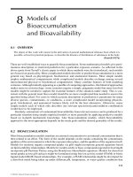
Dissimilarity among locations or between time points can also be used to evaluate responses to
environmental stressors. Philippi et al. (1998) quantified spatial and temporal responses to perturbations by comparing the pairwise dissimilarity between sites with the average dissimilarity among
replicate samples. These researchers noted that measures of dissimilarity (or similarity) can be
employed to evaluate changes in community composition during recovery (Figure 24.4). If remediation was effective, the relative dissimilarity between reference and impacted sites would be expected
to decrease over time.

1

0.8

0.6

0.4

0.2

0

0

1

2

3

4

5

6

7

Time since remediation

FIGURE 24.4 Hypothetical changes in community similarity between reference and impacted sites as
a function of time since remediation was initiated. The relationship shows that the index of dissimilarity
(expressed as the ratio of dissimilarity between sites to the average dissimilarity among sites) is reduced over
time as a result of remediation.

Clements: “3357_c024” — 2007/11/9 — 18:34 — page 480 — #8


Application of Multimetric and Multivariate Approaches in Community Ecotoxicology

481

While similarity indices provide a simple way to compare community composition, there are
potential problems with these measures. Boyle et al. (1990) evaluated the ability of similarity indices
to discriminate effects of simulated perturbations based on initial community structure, sensitivity
to community change, stability in response to reduced richness and abundance, and consistency.
These researchers concluded that some similarity indices were misleading because results were
strongly influenced by initial community composition and the nature of the perturbation. Although
similarity indices are useful when comparing communities from two locations, more sophisticated
techniques are necessary to compare multiple sites. Cluster analysis, a logical extension of similarity indices, is applicable for comparing communities from several locations or for comparing

the similarity of a single site with a group of sites. Cluster analysis employs a variety of similarity measures based on either presence–absence or abundance data. These data are often expressed
using a dendrogram, with the most similar sites combined into a single cluster. Additional sites are
included based on their similarity to the existing clusters. Several different clustering algorithms
have been developed, and relatively simple software packages are available for most analyses.
Details of the different clustering techniques and the justification for deciding how different sites
and clusters should be joined have been published (Gauch 1982). These methods will be described
below.

24.3.2 ORDINATION
Ordination is a process in which a large set of variables is reduced to a few variables with the intent of
enhancing conceptual parsimony and tractability. With ordination analysis of community abundance
data, the measured variables (e.g., abundance of each species for each sampling unit) are used to
identify hidden patterns or unmeasured factors explaining the data structure. Mathematical constructs
are sought to help interpret correlations among variables. There are five steps to ordination analysis,
regardless of the specific method applied (Comrey 1973). (1) The relevant data are generated and
selected for analysis. As noted above, the data might require transformation prior to use. (2) The
correlation matrix for the variables is calculated. (3) Factors (mathematical functions) are extracted.
(4) The factors might be rotated to enhance interpretation. (5) The factors are then interpreted. Ideally,
plots of the sampling unit positions along the first few mathematical constructs reveal explanatory,
or at least consistent, themes.
As an example, linear functions can be defined such as
Function 1 = b1 X1 + b2 X2 + b3 X3 + b4 X4 + · · · ,

(24.3)

where Xi = the normalized ln(abundance + 1) for each species sampled at the site. A first function
is constructed that incorporates as much of the variance in the data as possible, and the process is
repeated for additional functions with the remaining variance. Residual correlations after extraction
of the first factor are used to produce a second, uncorrelated function that explains as much of the
remaining variance as possible. The process is repeated to produce a series of functions. Ideally, most

of the variance will be explained in the first few functions. A score for each sampling unit can be
calculated for placement along each function. Plots for all sampling units using the formulated
functions as axes should reveal an interpretable pattern. In this process, a matrix of many species
abundances is reduced to a few sampling unit positions on a two- or three-dimensional plot. For
example, the entire species abundance data set for a site might be reduced to one point in a two- or
three-dimensional plot. The X, Y , and perhaps, Z dimensions are constructs that can be given physical
meaning such as the influences of soil type (Function 1), heavy metal contamination (Function 2),
and agricultural activity (Function 3) (Figure 24.5). Insight from additional information on soils,
agricultural history, and soil metal concentrations might be used to interpret the distribution of the
sampled plant communities along these three functions. The magnitude and signs of the b values
(loading coefficients) in the linear functions are used to identify an underlying theme for each axis.

Clements: “3357_c024” — 2007/11/9 — 18:34 — page 481 — #9


Ecotoxicology: A Comprehensive Treatment

482

Agriculture

Grasslands with few
metal-tolerant species
Grasslands with numerous
metal-tolerant species

So

il q

ua

lity

tals

Function 3

Me

on

2

ti
nc

Fu

Function 1

FIGURE 24.5 A hypothetical ordination analysis of plant communities relative to heavy metal contamination
(top panel). Abundances of species are quantified at five sites near abandoned mines and another eight reference
sites. Soil qualities and the history of agricultural use of the sites are also noted as potential confounding
factors. After data transformation, ordination analysis results in three orthogonal, linear functions that are
assigned interpretations of the influence of soil quality, soil metal concentrations, and agricultural history. The
five mine sites clearly cluster away from the reference sites. There is a gradient of communities relative to soil
quality and agricultural history. Ordination axes can be rotated to enhance interpretation using orthogonal and
oblique methods (bottom panel).

These loadings represent the extent to which the variables are related to the hypothetical factor.
For most factor extraction methods, these loadings may be thought of as correlations between the
variables and the function (Comrey 1973). For example, very high loadings in Function 2 for
species known to be tolerant to toxic metals and low or negative loadings for metal-sensitive species
would suggest the influence of metal exposure on community composition. For Function 3, high
loadings for species known to flourish in active agricultural areas might suggest the impact of active
agriculture on community structure. The final result at this stage for ordination analyses would be to
construct a table with rows of variables and associated loadings for each relevant factor (i.e., a table
of unrotated factor loadings).
Several types of ordination methods exist (Boxes 24.1 and 24.2). PCA was the first, and remains
the most popular method (Sparks 2000, Sparks et al. 1999). Using PCA, linear combinations of
the original variables are extracted that sequentially account for the residual variance in a series of
orthogonal (uncorrelated) components. The first component contains the most variance; the second

Clements: “3357_c024” — 2007/11/9 — 18:34 — page 482 — #10


Application of Multimetric and Multivariate Approaches in Community Ecotoxicology

Box 24.1

483

Pollution’s Signature on the Diversity of Estuarine Benthic Communities

To assess the influence of pollution on estuarine benthos, Diaz (1989) plotted species diversity
on principal component axes generated from physical and chemical data for several James River
(Virginia, USA) locations. Admittedly, one might object to this example because ordination is
not being used directly to summarize community data. However, the study is a good illustration of applying two multivariate methods to interpret pollution effects on communities. The
direct application of ordination to species abundance data will be described in Box 24.2 after

illustrating key aspects of ordination analysis with this example.
The challenge faced by Diaz (1989) was to assess the influence of pollution on benthic communities relative to several other confounding variables. Stations were sampled at 5 nautical
mile intervals from the fall line to within 10 miles of the river’s mouth. Factors potentially
influencing the benthic communities were measured, including sediment qualities, site-specific
point discharges, and general water quality characteristics. Prior to ordination analysis, sites
at salinity extremes were omitted to eliminate this obvious factor with a strong influence on
community diversity.
Ordination analysis of physical and chemical data from James River sites was done after
normalizing data with the formula
Zij =

Xij − Mj
,
SDj

(24.4)

where Zij = the standardized score of a datum for the jth variable of the ith site, Xij = the datum
for the jth variable for the ith site, and Mj and SDj = the mean and standard deviation of the data
for the jth variable, respectively. The normalized data were analyzed by principal components
methods with no mention of any rotation of axes. Whether or not a rotation procedure would
have produced more parsimonious principal components remains ambiguous.
Table 24.1 summarizes the PCA results. The percentage of total variance accounted for
by each of the first five principal components is provided at the top of the table. Loadings
(eigenvectors) for each chemical or physical factor are given for each principal component with
TABLE 24.1
Loadings (Eigenvectors) for Five Principal Components Derived by Diaz (1989)
for James River Physical and Chemical Data
Principal Component
Percentage of total variance (%)

Discharge biochemical oxygen demand
Discharge chemical oxygen demand
Discharge coliform bacteria
Discharge total suspended solids
Ammonia concentration in water
Nitrite/nitrate concentration in water
Phosphate in water
Suspended solids in water
Biochemical oxygen demand in water
Number of discharges
Percentage silt and clay
Cross-sectional area

1
36
0.33
0.24
0.31
0.23
0.13
−0.14
0.32
−0.23
0.39
0.32
−0.19
−0.36

2
22

0.37
0.46
−0.09
−0.19
0.02
0.49
−0.30
0.33
0.14
0.31
−0.11
0.18

3
15
0.00
−0.07
0.23
−0.02
−0.13
−0.26
0.16
0.25
−0.02
−0.01
−0.60
0.15

4
12

0.20
0.20
0.04
0.10
−0.70
−0.20
−0.10
−0.37
−0.32
0.28
0.13
0.20

5
8
0.05
0.16
−0.58
0.73
0.03
−0.03
−0.07
0.00
0.00
−0.17
−0.10
−0.02

Note: Boldface Indicates a variable with high loading.

Clements: “3357_c024” — 2007/11/9 — 18:34 — page 483 — #11


Ecotoxicology: A Comprehensive Treatment

484

1.46
1.86
1.60

2.01

FIGURE 24.6 Ordination analysis (PCA) of
physical and chemical qualities at sites along
the James River (Virginia). Axes One and Two
were interpreted as municipal waste discharge
and industrial waste discharge, respectively.
Numbers at each river site position on the plot
are species diversities (H ). (Modified from
Figure 7 of Diaz (1989).)

2.42

2.48

Axis two

2.53
2.81

2.46
2.71

3.24

Axis one

large eigenvectors in boldface. The large eigenvectors for specific variables in the first, fourth,
and fifth principal components suggested to Diaz (1989) that these principal components
reflected municipal waste discharges. Those variables with large eigenvectors in the second
principal component suggested industrial discharges. The third principal component seemed to
be related to physical characteristics of sediments.
The first two principal components were used as axes for plotting species diversity at the
different sampling sites (Figure 24.6). Assuming the correct interpretation of the first principal
component, an increase in municipal waste discharge was clearly associated with a decrease
in species diversity (H ). The authors concluded from the plot that, “the greater the pollution
load the lower the species diversity.”

Box 24.2

Pesticide Spraying Changes Mesocosm Communities

Kedwards et al. (1999a,b) used ordination to study the impact of the pyrethroid pesticides,
cypermethrin and lambda-cyhalothrin, on benthic communities established in 30-m3 artificial ponds. Treatment involved duplicate mesocosms that were sprayed every 2 weeks
for a total of four sprayings per mesocosm. Preapplication data were collected 5 weeks
before the first spraying and sampling continued for 14 weeks after the final spraying
occurred.
Redundancy analysis, an ordination technique, was applied to the results from cypermethrinsprayed mesocosms (Figure 24.7). The two axes used in this figure accounted for 54% and 14%
of the total variance in the data. Immediately after spraying began, the community in the treated

mesocosms diverged from that of the controls, and each successive spraying moved the treated
community further away. Several months after the last spraying, the communities remained
quite divergent.
The authors interpreted the first two axes as being the influence of cypermethrin spraying
(axis one) and the temporal changes in species abundances (axis two). The lines describing
temporal changes in the reference mesocosms moved up and down along the second axis, but
remained constant in its position relative to the first axis. The communities in the sprayed
mesocosms changed with time and with spraying treatment. Spraying shifted community
composition further to the right along the first axis, reflecting an increase in abundance of
Chironomidae, Planorbidae, Hirudinea, and Lymnaeidea, and a decrease in Gammaridae and
Asellidae.

Clements: “3357_c024” — 2007/11/9 — 18:34 — page 484 — #12


Application of Multimetric and Multivariate Approaches in Community Ecotoxicology

485

Axis two

X
S

X

Axis one

X

Temporal change in cypermethrin-spiked
community composition
Temporal change in unspiked
community composition
S

Designates first sample after spraying

X

Designates biweekly dosing

FIGURE 24.7 Ordination results for benthic
invertebrate community composition for reference and cypermethrin-sprayed mesocosms.
Community composition shifted abruptly along
axis one at the sampling after spraying (denoted
as S on diagram). Axis one and two were interpreted as the effect of spraying and the effect of
time on community composition, respectively.
(Modified from Figure 2 in Kedwards et al.
(1999b).)

contains the most of the residual variance, and so forth. Ideally, the first few principal components
account for most of the variance and the loadings allow sensible interpretations of these components.
If this is not the case, some rotation method might be required.
Another general ordination method, factor analysis, is similar to PCA in that the variables are
used to produce linear functions. Instead of being called principal components, these linear functions
of the data are called factors. A factor is an unobservable variable that has attributes of a subset of
the observed variables. In contrast to PCA in which components are calculated directly as linear
functions of the observed variables, the observed variables in factor analysis are envisioned as linear
functions of the factors (unobserved variables) plus random error (Sparks et al. 1999).

Numerous other ordination methods are available for applications with specific needs. Ordination can be done with discrete data using correspondence analysis or detrended correspondence
analysis (Sparks et al. 1999). Discrete data might consist of presence/absence information or categorized species abundances such as rare, uncommon, common, abundant, or dominant. Although
most multivariate ordination approaches employ traditional measures of community composition
(e.g., abundance, presence/absence of species), other metrics may be necessary for groups where
taxonomic issues limit our ability to identify species. Cao et al. (2006) used multivariate ordination
to assess how bacterial community composition, as determined by phospholipid fatty acid and terminal restriction fragment length polymorphism analyses, responded to a mixture of contaminants.
Nonmetric ordination methods exist (see Sparks 2000 for details) and have been used successfully
to describe insect communities exposed to NEEM products (Kreutzweiser et al. 2000), Norwegian
oilfield macrofauna (Clarke 1999), and benthic macroinvertebrates of the River Tees (Crane et al.
2002).
Methods for extracting functions aim to produce easily interpretable patterns. The mathematical
functions or axes that are initially generated are uncorrelated or perpendicular. To enhance interpretation of these functions, some methods will rotate the axes at this stage of analysis based on some
particular set of rules or criteria. Axes remain uncorrelated with orthogonal rotations but become
correlated with oblique rotations. Many rotation methods are available for ordination; however,
there is no formal statistical approach for determining which is best, and selection is usually based
on user preferences. Among the most widely used rotation methods, the Kaiser Varimax produces

Clements: “3357_c024” — 2007/11/9 — 18:34 — page 485 — #13


Ecotoxicology: A Comprehensive Treatment

486

orthogonal functions with as few variables with intermediate loadings as possible (Kaiser 1958,
1959, see also Comrey 1973). The concept is that a function with a few variables with very high or
very low loadings will be more easily interpretable or parsimonious than one with many variables
with intermediate loadings.

24.3.3 DISCRIMINANT AND CLUSTER ANALYSIS

Some multivariate methods, such as cluster and canonical discriminant analysis, explore differences
or distances between sampling units. Groups for which differences are being assessed might be
defined by the researcher (e.g., communities from polluted vs. clean sites), by design (e.g., treatment levels of copper added to a series of microcosms), or by statistical methods (e.g., community
groupings identified by cluster analysis). Discriminant analysis aims to develop quantitative rules for
separating groups or classes of sampling units. Similar to PCA, some discriminant analysis methods
generate functions (canonical variates) that produce maximum discrimination among sampling units.
Loading coefficients associated with the different variables suggest which variables contribute the
most to the differences among sampling units (Box 24.3).

Box 24.3
Groups?

Copper-Exposed Communities: What Separates Treatment

A series of triplicate 17-m3 freshwater microcosms were spiked at 5 copper levels in an effort
to define techniques for determining differences among toxicant-treated communities (Shaw
and Manning 1996). In situ bioassays and species abundance data were collected, but only
canonical discriminant analysis of macroinvertebrate species abundance data are presented
here. Canonical variables, linear combinations of species abundance data that best distinguished among treatments, were produced for a series of times during the trial. Analysis
for one sampling date during the spiking period (August 31, 1 month after spiking began
and 19 days after the last spiking) is provided in Figure 24.8. The results show clear separation among treatments based on community composition. Surprisingly, species richness was
not affected by copper spiking. However, abundances of annelids, crustaceans, mayflies, and
chironomids did change. The mayfly Caenis was primarily responsible for separation among
spiked treatments along the first canonical axis. (Importantly, Caenis bioassays in the spiked
microcosms were also among the most useful for measuring effects of copper.) Orthocladiinae,

4
1

FIGURE 24.8 Separation of macroinvertebrate communities of microcosms receiving different copper treatments (spiked amounts being

ranked as control < 1 < 2 < 3 < 4 < 5).
Results are those obtained for canonical discriminant analysis of species abundance data
for the August 31 sampling. The three observations plotted for each treatment are those for the
triplicate microcosms. (Modified from Figure 8
of Shaw and Manning (1996).)

4
4

5

33 3

Canonical variable 1

1
C

2
5

5

C

1C

2
2

Canonical variable 2

Clements: “3357_c024” — 2007/11/9 — 18:34 — page 486 — #14


Application of Multimetric and Multivariate Approaches in Community Ecotoxicology

487

Chironominae, and Hydrozetes were also important. Only four taxa were needed to separate
groups along copper treatments, suggesting that these species are useful indicators of metal
pollution.

Cluster analysis also distinguishes among sampling units using multivariate data sets. As discussed in detail by Ludwig and Reynolds (1988) and Matthews et al. (1998), diverse metrics of
resemblance or distance are applied to sampling units. Sampling units may be grouped in a hierarchical or nonhierarchical manner using a variety of algorithms. Hierarchical schemes produce tree-like
structures (dendrograms) with branching points along groupings suggesting the degree of distinction or similarity among the groups on the various branches. Nonhierarchical methods simply place
sampling units into groupings. Sparks et al. (1999) give the example of K-means clustering in which
the number of groups is defined prior to analysis and the sampling units are sorted optimally into
these groups. Using this method, differences are quantified as the square of the Euclidean distance
(Matthews et al. 1998) and sampling units are distributed among the groups to produce maximum
group separation.
Cluster analysis has many applications in community ecotoxicology. For example, Matthews
et al. (1996) used nonmetric clustering (Matthews et al. 1995) to study microcosm community
structural changes after turbine fuel exposure. The clustering methods revealed that differences
among treated microcosms persisted for long periods of time, leading the authors to propose the
community-conditioning hypothesis described in Chapter 25. In a field setting, Dauer et al. (1992)
used cluster analysis to group benthic communities according to the influence of several physical
and water quality characteristics (Box 24.4).

Box 24.4

Cluster Analysis Identifies Benthic Communities Affected by Anoxia

Physical and chemical qualities within estuaries greatly influence the composition of benthic
communities. Dauer et al. (1992) explored Lower Chesapeake Bay (USA) benthic communities in an attempt to quantify the influence of such factors on community structure. Emphasis
was placed on identifying communities modified by episodes of anoxia. Benthic species are
subjected to anoxia when water produced during seasonal stratification is moved onto nearby
shallows by wind-driven seiches. The extent and effect of anoxia are of concern because of
potential exacerbation by increased nutrient influx from human activities.
Twenty-one samples were taken along the Lower Chesapeake Bay and in several tributaries. Water quality data, including oxygen concentrations, were available for interpreting benthic
species abundance information. Site selection intentionally included those along salinity gradients, those with different sediment types, and those that experienced episodic anoxia. Cluster
analysis was done using logarithm-transformed species abundance data and the Bray-Curtis
similarity coefficient.
Cluster analysis identified groupings that were easily interpreted based on salinity, sediment type, and dissolved oxygen concentration (Figure 24.9). For explanatory convenience,
six clusters are identified in Figure 24.9. There was a clear clustering of sites relative to salinity: freshwater (Cluster 6), transitional (Cluster 5), mesohaline (Cluster 4), and polyhaline
(Clusters 2 and 3) sites. Within the polyhaline grouping, the communities split again into those
associated with sandy (Cluster 2) and muddy (Cluster 3) substrates. Sites experiencing anoxia
(four sites in Cluster 1) were set apart from the other sites (17 sites in Clusters 2 through 6) at
a relatively high level (e.g., similarity of approximately 0.9). Relative to the other communities
sampled, those experiencing periodic anoxia had lower species diversity, lower biomass, and

Clements: “3357_c024” — 2007/11/9 — 18:34 — page 487 — #15


Ecotoxicology: A Comprehensive Treatment

488

Similarity

1.5

1.0

0.5

1

2

3

5

4

6

0.0

FIGURE 24.9 Clustering of 21 benthic
macroinvertebrate communities based on BrayCurtis similarity coefficient. The clustering was
interpreted by applying knowledge of salinity,
oxygen, and sediment conditions. (Modified
from Figure 2 of Dauer et al. (1992).)

Hypoxia

No hypoxia
Oxygen regime

Sandy
Mud
Bottom type
Polyhaline

Mesohaline

Transitional

Freshwater

Salinity regime

less biomass deeper than 5 cm in the sediments. Results also showed that dominant species
tended to be opportunistic, with equilibrium species being less common than in the other
communities.

24.3.4 APPLICATION OF MULTIVARIATE METHODS TO
LABORATORY DATA
With minor exceptions, most of the multivariate methods described to this point draw from species
enumerations in order to describe community-level responses. However, other multivariate methods
use results of single species toxicity tests to predict effects on communities. Box 24.5 describes
an example that uses laboratory toxicity data for sediment and water to make predictions about
community status.

Box 24.5

A Risk Ranking Model Based on Estuarine Fish Communities

The Maryland Department of Natural Resources (USA) developed a composite index (risk

ranking) for Chesapeake Bay tributaries (Hartwell 1997, also see Hartwell et al. 1997) using
laboratory toxicity tests of water and sediments from sites of interest. The intent was to initially
“quantify the toxicological risk to populations due to the presence of toxic contamination . . .”
using ambient toxicity data. (See Newman (1998, 2001) for discussion of the problems in predicting population consequences based on these types of severity judgments.)
Four estuaries were selected to estimate a fish community-based IBI, fish species diversity,
and this new ranking model. The ranking model employed water and sediment test results to
quantify region status. On several dates, water samples from each site were collected for ambient toxicity tests, including sheepshead minnow (Cyprinodon variegatus) growth and survival,
grass shrimp (Palaemonetes pugio) growth and survival, and copepod (Eurytemora affinis)
reproduction and survival. Similarly, sediment toxicity tests were done including those quantifying sheepshead minnow embryo-larval survival and teratogencity, amphipod (Leptocheirus
plumulosus) reburial, growth, and survival, and polychaete (Streblospio benedicti) survival and
growth.
This ranking system of risk was influenced by a high hazard score for a particular measure
and the uncertainty associated with producing a score for a region. The level of uncertainty

Clements: “3357_c024” — 2007/11/9 — 18:34 — page 488 — #16


Application of Multimetric and Multivariate Approaches in Community Ecotoxicology

489

influenced the score and the measured level of hazard. The severity of effect (mortality = 3,
impaired reproduction = 2, impaired growth = 1), degree of response, variability in testing,
site consistency, and the number of endpoints were components of the risk ranking model.
The degree of response was the proportional difference from the control. The variability was
expressed as the coefficient of variation (CV) for a particular metric for each set of laboratory
replicates and each sample site during a particular sampling period. The last part of the ranking
model involved consistency, or the level of agreement among assays for a site. Consistency was
quantified as the cube root of the difference between half of the number of tests (N/2) and the
number of statistically nonsignificant responses at each site (X):

Consistency =

3

N/2 − X.

(24.5)

The consistency is then divided by the number of endpoints measured for a site. The site
score is estimated with the following equation:
Location score =

(severity × response × CV) + consistency
.
√
N

(24.6)

Scores were calculated for the four sites based on tests of water alone, sediment alone, or
water and sediment combined. Pearson correlation coefficients were calculated for these scores
versus a fish-based IBI, a benthic species diversity index, and a resident fish diversity index.
There were no significant correlations (α = 0.05) between the risk scores (water, sediment,
or water sediment combined) and the IBI scores or species diversity based on all resident fish
species. Similarly, no significant correlation was noted between water testing-based risk scores
and bottom fish species diversity. However, there were significant correlations between bottom
fish species diversity and the sediment test-based risk score (P = .0092) and the combined
test risk score (P = .0018). These results suggest that scores for this risk index are related to
bottom fish diversity. Notionally, the relationship involved responses to site-associated toxicant
exposures.

The methods described to this point have involved data collected from potentially impacted sites
in an attempt to document community changes. However, species sensitivity distribution (SSD) methods use mostly laboratory data to predict potential community changes on exposure to stressors. The
approach extends the common use of one laboratory measure of effect, such as the 96-h LC50, to
predict impact to an exposed community. Conventional prediction from one species can be made
more credible by making predictions of effect based on information from the most sensitive test
species. The SSD method modifies these laboratory-based approaches by using all available laboratory data to make predictions of effect concentrations for the ecological community. Its greatest
advantage is that it uses all of the readily available information to predict community consequences.
Its convenience and efficient use of single species data have led to a very rapid increase in its use
(Newman 1995).
To apply the SSD method, effect concentrations such as acute LC50 or no-observed effect concentration (NOEC) values are collected for all relevant species. The effect concentration observations
are ordered from the smallest to the largest value (e.g., smallest to largest 96-h LC50 values). The
ordered values are then given a rank using one of several conventional methods. Currently popular is
i/(n + 1), where i = the ith ranked observation and n = the total number of observations. A slightly
better, but less commonly applied, approximation of rank for ordered observations is (i − 0.5)/n. At
this point, the data set consists of a series of observations (e.g., 96-h LC50 observations and their
corresponding ranks). A log normal model is often assumed and the probit transformation of each
rank is taken. Another model and transformation can be used if there is evidence that the log normal

Clements: “3357_c024” — 2007/11/9 — 18:34 — page 489 — #17


Ecotoxicology: A Comprehensive Treatment

Probit of rank

490

Log of HCp
Log of effect concentration

FIGURE 24.10 Log normal model for estimating the HCp using the SSD method. Transformations are easily
done on effect concentrations and effect proportion in order to linearize species sensitivity data. The log of the
effect concentration is plotted against the probit of the effect proportion for the log normal model assumed here.

model is inappropriate. Newman et al. (2000, 2001) indicate that the general assumption of a log
normal model is often not appropriate. Regardless, a log normal model will be assumed here to illustrate the SSD method. A plot of logarithm of effect concentration versus probit of the rank is made,
producing a straight line (Figure 24.10) if the log normal assumption is appropriate. A regression
model is then used to estimate the concentration “protecting” all but a specified percentage (p%) of
species in the community. This concentration is often called the hazard concentration or HCp .
Although the SSD approach enjoys increasingly widespread application (Posthuma et al. 2001),
it does involve several unresolved shortcomings or ambiguities (Newman 2001, Newman et al.
2000). First, EC50, LC50, NOEC, lowest-observed effect concentration (LOEC), and maximum
allowable toxicant concentration (MATC) effects metrics are used to generate models but they have
significant deficiencies as predictors of population persistence in natural communities. Any HCp
derived using these effects metrics will consequently have deficiencies as a predictor of community
consequences. Second, the selection of a specified p implies that some loss of species is acceptable for
any community because of species redundancy. As will be described in Chapter 25, the extent to which
this redundancy hypothesis can be validly applied is still hotly debated. Therefore, any predictions
based on the redundancy hypothesis must be viewed as nonconservative predictions at this time.
Third, application of the SSD method requires thorough knowledge of the dominant and keystone
species, and the importance of species interactions. It has been our experience that this knowledge
is often not available in studies applying the SSD method. Fourth, in situ exposure is more complex
and species-dependent rather than reflected in the laboratory exposures done in toxicity testing.
Fifth, there is a bias toward lethality information, although nonlethal effects can result in species
disappearance from a community. Finally, the assumption of a specific model, such as the log normal
model, is often made without careful scrutiny (Jagoe and Newman 1997, Newman et al. 2000, 2001).

24.3.5 TAXONOMIC AGGREGATION IN MULTIVARIATE ANALYSES
Our previous discussion in Chapter 22 concerning how taxonomic aggregation and the exclusion
of rare taxa influence our ability to distinguish reference and contaminated sites is also relevant to

multivariate analyses. Ordination approaches are typically based on responses of individual species
to environmental gradients. In fact, the argument frequently used to support these techniques is
that multivariate approaches allow researchers to quantify the response of an entire community.
However, depending on the degree of interspecific variation in sensitivity, there is likely some degree

Clements: “3357_c024” — 2007/11/9 — 18:34 — page 490 — #18


Application of Multimetric and Multivariate Approaches in Community Ecotoxicology

491

of redundancy in the responses of individual taxa to contamination. From a practical perspective, the
complex taxonomy of some groups severely limits species-level identification. Caruso and Migliorini
(2006) showed that multivariate analyses based on either genus- or family-level identification could
detect effects of heavy metals on soil invertebrate communities. While these results are certainly
encouraging, it is important to note that the loss of information associated with taxonomic aggregation
may vary among groups. For example, Hirst (2006) showed that family-level identification was
sufficient to identify multivariate patterns in marine invertebrates, but taxonomic aggregation of
macroalgae resulted in a significant reduction in information.

24.4 SUMMARY
In summary, a diverse array of analytical approaches allows for the description of toxicant effects
on communities. Some, such as species diversity indices, reduce abundance data to a single number
while others, such as the IBI, apply considerable ecological knowledge to generate ad hoc measures
of community integrity. Others, like the SSD approach, attempt to use available laboratory data to
produce gross predictions of possible community-level effects. Finally, multivariate procedures are
devoid of ecological theory and simply identify correlations or associations within a data set. All of
these approaches can be extremely useful for detecting community differences or changes if applied
insightfully.

24.4.1 SUMMARY OF FOUNDATION CONCEPTS AND PARADIGMS
• Methods to assess the effects of contaminants on communities range from computationally
simple indices such as species richness to complex, computer-dependent algorithms such
as multivariate analyses.
• The simplest community indices use species presence/absence or abundance data to show
how individuals in the community are distributed among species.
• Computationally intense methods, such as multivariate analyses, aim to reduce the number of data dimensions to an interpretable low number, and to quantify similarities or
differences among sampling units.
• One of the most significant advances in the field of biological assessments over the past
20 years was the development and application of multimetric approaches for measuring
ecological integrity.
• The individual metrics in a multimetric index reflect different characteristics of life history,
community structure, and functional organization that are integrated into a single measure.
• Karr’s (1981) IBI is the most widely used multimetric index for assessing the health of
aquatic communities.
• Similarity indices reduce complex, multispecies data and quantify correspondence
between two communities based on either presence–absence or abundance.
• In contrast to multimetric indices, multivariate analyses are not based on ecological concepts but are statistical constructs that reduce complex data sets to illustrate potentially
meaningful patterns involving a few variables.
• Multivariate data sets are broadly defined as those in which more than two dependent or
independent variables are collected for each sampling unit.
• Ordination is a process in which a large set of variables is reduced to a few variables with
the intent of enhancing conceptual parsimony and tractability.
• In PCA, linear combinations of the original variables are extracted to sequentially account
for the residual variance in a series of orthogonal (uncorrelated) components.
• Nonmetric ordination methods have been used successfully to describe macroinvertebrate
responses to a variety of contaminants.

Clements: “3357_c024” — 2007/11/9 — 18:34 — page 491 — #19

Ecotoxicology: A Comprehensive Treatment

492

• Some multivariate methods, such as cluster and canonical discriminant analysis, explore
differences or distances between sampling units.
• Discriminant analysis develops quantitative rules for separating groups or classes of
sampling units either defined by the researcher (e.g., communities from polluted vs.
clean sites), by experimental design (e.g., treatment levels of copper added to a series of
microcosms), or by statistical methods (e.g., community groupings identified by cluster
analysis).
• Cluster analysis distinguishes among sampling units using multivariate data sets grouped
in a hierarchical or nonhierarchical manner using a variety of algorithms.
• Despite their growing popularity, multivariate approaches have been criticized because of
their inherent statistical complexity and because results are often difficult to interpret.
• Although strict reliance on complex statistical algorithms may obscure important biological results, multivariate approaches are an essential set of tools for assessments of water
quality.
• Multivariate and multimetric approaches are complementary and should be used in conjunction. Variables used in multivariate analyses could include species richness, abundance
of sensitive groups, or other measures typically included in a multimetric index. Alternatively, a multimetric index similar to Karr’s IBI could be developed using results of
multivariate analyses.

REFERENCES
Bailey, R.C., Kennedy, M.G., Dervish, M.Z., and Taylor, R.M., Biological assessment of freshwater ecosystems
using a reference condition approach: Comparing predicted and actual benthic invertebrate communities
in Yukon streams, Freshw. Biol., 39, 765–774, 1998.
Blair, R.B., Birds and butterflies along an urban gradient: Surrogate taxa for assessing biodiversity? Ecol. Appl.,
9, 164–170, 1999.
Boyle, T.P., Smillie, G.M., Anderson, J.C., and Beeson, D.R., A sensitivity analysis of nine diversity and seven

similarity indices, Water Poll. Con. Fed., 62, 749–762, 1990.
Cao, Y., Cherr, G.N., Cordova-Kreylos, A.L., Fan, T.W.M., Green, P.G., Higashi, R.M., Lamontagne, M.G.,
et al., Relationships between sediment microbial communities and pollutants in two California salt
marshes, Microb. Ecol., 52, 619–633, 2006.
Caruso, T., and Migliorini, M., Micro-arthropod communities under human disturbance: Is taxonomic aggregation a valuable tool for detecting multivariate change? Evidence from Mediterranean soil oribatid
coenoses, Acta Oecol.-Int. J. Ecol., 30, 46–53, 2006.
Chambers, C.L., McComb, W.C., and Tappeiner, J.C., I., Breeding bird responses to three silvicultural treatments
in the Oregon Coast Range, Ecol. Appl., 9, 171–185, 1999.
Chenery, A.M. and Mudge, S.M., Detecting anthropogenic stress in an ecosystem: 3. Mesoscales variability
and biotic indices, Environ. Foren., 6, 371–384, 2005.
Clarke, K.R., Nonmetric multivariate analysis in community-level ecotoxicology, Environ. Toxicol. Chem., 18,
118–127, 1999.
Clements, W.H. and Kiffney, P.M., The influence of elevation on benthic community responses to heavy metals
in Rocky Mountain streams, Can. J. Fish. Aquat. Sci., 52, 1966–1977, 1995.
Clements, W.H., Cherry, D.S., and Cairns, J., Jr., The impact of heavy metals on macroinvertebrate communities:
A comparison of observational and experimental results, Can. J. Fish. Aquat. Sci., 45, 2017–2025,
1988.
Comrey, A.L., A Course in Factor Analysis, Academic Press, New York, 1973.
Crane, M., Sorokin, N., Wheeler, J., Grosso, A., Whitehouse, P., and Morritt, D., European approaches to
coastal and estuarine risk assessment, In Coastal and Estuarine Risk Assessment, Newman, M.C.,
Roberts, M.H. Jr., and Hale, R.C. (eds.), CRC Press, Boca Raton, FL, 2002, pp. 15–39.
Dauer, D.M., Rodi, A.J., Jr., and Ranasinghe, J.A., Effects of low dissolved oxygen events on the macrobenthos
of the Lower Chesapeake Bay, Estuaries, 15, 384–391, 1992.

Clements: “3357_c024” — 2007/11/9 — 18:34 — page 492 — #20


Application of Multimetric and Multivariate Approaches in Community Ecotoxicology

493

Diaz, R.J., Pollution and tidal benthic communities of the James River Estuary, Virginia, Hydrobiologia, 180,
195–211, 1989.
Fausch, K.D., Lyons, J., Karr, J.R., and Angermeier, P.L., Fish communities as indicators of environmental
degradation, Am. Fish. Soc. Symp., 8, 123–144, 1990.
Fore, L.S., Karr, J.R., and Wisseman, R.W., Assessing invertebrate responses to human activities: Evaluating
alternative approaches, J. N. Am. Benthol. Soc., 15, 212–231, 1996.
Gauch, H.G., Jr., Multivariate Analysis in Community Ecology, Cambridge University Press, Cambridge,
England, 1982.
Gerritsen, J., Additive biological indices for resource management, J. N. Am. Benthol. Soc., 14, 451–457,
1995.
Griffith, M.B., Husby, P., Hall, R.K., Kaufmann, P.R., and Hill, B.H., Analysis of macroinvertebrate assemblages
in relation to environmental gradients among lotic habitats of California’s Central Valley, Environ.
Monitor. Assess., 82, 281–309, 2003.
Hartwell, S.I., Demonstration of a toxicological risk ranking method to correlate measures of ambient toxicity
and fish community diversity, Environ. Toxicol. Chem., 16, 361–371, 1997.
Hartwell, S.I., Dawson, C.E., Durell, E.Q., Alden, R.W., Adolphson, P.C., Wright, D.A., Coehlo, G.M.,
Magee, J.A., Ailstock, S., and Norman, M., Correlation of measures of ambient toxicity and fish
community diversity in Chesapeake Bay, USA, tributaries—urbanizing watersheds, Environ. Toxicol.
Chem., 16, 2556–2567, 1997.
Hirst, A.J., Influence of taxonomic resolution on multivariate analyses of arthropod and macroalgal reef
assemblages, Mar. Ecol. Prog. Ser., 324, 83–93, 2006.
Jagoe, R.H. and Newman, M.C., Bootstrap estimation of community NOEC values, Ecotoxicology, 6, 293–306,
1997.
Kaiser, H.F., The Varimax criterion for analytic rotation in factor analysis, Psychometrika, 31, 313–323,
1958.
Kaiser, H.F., Computer program for Varimax rotation in factor analysis, Ed. Psych. Meas., 19, 413–420,
1959.
Karr, J.R., Assessment of biological integrity using fish communities, Fisheries, 6, 21–27, 1981.
Karr, J.R., Defining and assessing ecological integrity: Beyond water quality, Environ. Toxicol. Chem., 12,

1521–1531, 1993.
Kedwards, T.J., Maund, S.J., and Chapman, P.F., Community level analysis of ecotoxicological field studies: I.
Biological monitoring, Environ. Toxicol. Chem., 18, 149–157, 1999a.
Kedwards, T.J., Maund, S.J., and Chapman, P.F., Community level analysis of ecotoxicological field studies: II.
Replicated-design studies, Environ. Toxicol. Chem., 18, 158–166, 1999b.
Kerans, B.L. and Karr, J.R., A benthic index of biotic integrity (B-IBI) for rivers of the Tennessee Valley,
Ecol. Appl., 4, 768–785, 1994.
Kilgour, B.W., Somers, K.M., and Barton, D.R., A comparison of the sensitivity of stream benthic community
indices to effects associated with mines, pulp and paper mills, and urbanization, Environ. Toxicol.
Chem., 23, 212–221, 2004.
Kremen, C., Assessing the indicator properties of species assemblages for natural areas monitoring, Ecol. Appl.,
2, 203–217, 1992.
Kremen, C., Colwell, R.K., Erwin, T.L., Murphy, D.D., Noss, R.F., and Sanjayan, M.A., Terrestrial arthropod
assemblages: Their use in conservation and planning, Conserv. Biol., 7, 796–808, 1993.
Kreutzweiser, D.P., Capell, S.S., and Scarr, T.A., Community-level responses by stream insects to NEEM
products containing azadirachtin, Environ. Toxicol. Chem., 19, 855–861, 2000.
Lewis, C.S., The Screwtape Letters, HarperCollins Publishers, Inc., New York, 1942.
Ludwig, J.A., and Reynolds, J.F., Statistical Ecology. A Primer on Methods and Computing, John Wiley &
Sons, New York, 1988.
Magurran, A.E., Ecological Diversity and Its Management, Princeton University Press, Princeton, NJ,
1988.
Matthews, G.M., Matthew, R., and Landis, W., Nonmetric conceptual clustering in ecology and ecotoxicology,
AI Appl., 9, 41–48, 1995.
Matthew, R.A., Matthew, G.M., and Landis, W.G., Application of community level toxicity testing to environmental risk assessment, In Risk Assessment. Logic and Measurement, Newman, M.C. and Strojan, C.L.
(eds.), CRC Press, Boca Raton, FL, 1998, pp. 225–253.

Clements: “3357_c024” — 2007/11/9 — 18:34 — page 493 — #21


494

Ecotoxicology: A Comprehensive Treatment

Matthews, R.A., Landis, W.G., and Matthews, G.B., The community conditioning hypothesis and its application
to environmental toxicology, Environ. Toxicol. Chem., 15, 597–603, 1996.
Miller, D.I., Leonard, M., Hughes, R.M., Karr, J.R., Moyle, P.B., Schrader, L.H., Thompson, B.A., et al.,
Regional applications of an index of biotic integrity for use in water resource management, Fisheries,
13, 12–20, 1988.
Nelson, S.M., and Epstein, M.E., Butterflies (Lepidoptera: Papilionoidea and Hesperioidea) of Roxborough
State Park, Colorado, USA: Baseline inventory, community attribute, and monitoring plan, Environ.
Manag., 22, 287–295, 1998.
Newman, M.C., Quantitative Methods in Aquatic Ecotoxicology, CRC Press, Boca Raton, FL, 1995.
Newman, M.C., Fundamentals of Ecotoxicology, CRC Press, Boca Raton, FL, 1998.
Newman, M.C., Population Ecotoxicology, John Wiley & Sons, Chichester, UK, 2001.
Newman, M.C., Ownby, D.R., Mezin, L.C.A., Powell, D.C., Christensen, T.R.L., Lerberg, S.B., and
Anderson, B.A., Applying species sensitivity distributions in ecological risk assessment: Assumptions of distribution type and sufficient numbers of species, Environ. Toxicol. Chem., 19, 508–515,
2000.
Newman, M.C., Ownby, D.R., MJzin, L.C.A., Powell, D.C., Christensen, T.R.L., Lerberg, S.B., Anderson, B.A.,
and Padma, T.V., Species sensitivity distributions in ecological risk assessment: Distributional assumptions, alternate bootstrap techniques, and estimation of adequate number of species, In Species
Sensitivity Distributions in Ecotoxicology, Posthuma, L., Sutter, G.W., II, and Traas, T.P. (eds.),
CRC Press, Boca Raton, FL, 2001, pp. 119–132.
Pardal, M.A., Cardoso, P.G., Sousa, J.P., Marques, J.C., and Raffaelli, D., Assessing environmental quality:
A novel approach, Mar. Ecol. Prog. Ser., 267, 1–8, 2004.
Philippi, T.E., Dixon, P.M., and Taylor, B.E., Detecting trends in species composition, Ecol. Appl., 8, 300–308,
1998.
Plafkin, J.L., Barbour, M.T., Porter, K.D., Gross, S.K., and Hughes, R.M., Rapid Bioassessment Protocols
for Use in Streams and Rivers: Benthic Macroinvertebrates and Fish. EPA 440/4-89-001, Washington,
D.C., U.S. EPA, 1989.
Posthuma, L., Suter, G.W., II, and Traas, T.P., Species Sensitivity Distributions in Ecotoxicology, CRC Press,
Boca Raton, FL, 2001.

Quintino, V., Elliott, M., and Rodrigues, A.M., The derivation, performance and role of univariate and multivariate indicators of benthic change: Case studies at differing spatial scales, J. Exp. Mar. Biol. Ecol.,
330, 368–382, 2006.
Resh, V.H., Norris, R.H., and Barbour, M.T., Design and implementation of rapid assessment approaches
for water resource monitoring using benthic macroinvertebrates, Aust. J. Ecol., 20, 108–121,
1995.
Reynoldson, T.B., Norris, R.H., Resh, V.H., Day, K.E., and Rosenberg, D.M., The reference condition: A comparison of multimetric and multivariate approaches to assess water-quality impairment using benthic
macroinvertebrates, J. N. Am. Benthol. Soc., 16, 833–852, 1997.
Shaw, J.L. and Manning, J.P., Evaluating macroinvertebrate population and community level effects in outdoor
microcosms: Use of in situ bioassays and multivariate analysis, Environ. Toxicol. Chem., 15, 608–617,
1996.
Simon, T.P. and Lyons, L., Application of the index of biotic integrity to evaluate water resource integrity
in freshwater ecosystems, In Biological assessment and criteria: Tools for water resource planning
and decision making, Davis, W.S. and Simon, T.P. (eds.), Lewis Publishers, Boca Raton, FL, 1995,
pp. 245–262.
Sparks, T.H., Statistics in Ecotoxicology, John Wiley & Sons, Chichester, UK, 2000.
Sparks, T.H., Scott, W.A., and Clarke, R.T., Traditional multivariate techniques: Potential for use in
ecotoxicology, Environ. Toxicol. Chem., 18, 128–137, 1999.
Suter, G.W., II, A critique of ecosystem health concepts and indexes, Environ. Toxicol. Chem., 12, 1533–1539,
1993.
Terlizzi, A., Scuderi, D., Fraschetti, S., and Anderson, M.J., Quantifying effects of pollution on biodiversity:
A case study of highly diverse molluscan assemblages in the Mediterranean, Mar. Biol., 148, 293–305,
2005.
Thomas, J.F., and Hall, T.J., A comparison of three methods of evaluating aquatic community impairment in
streams, J. Freshw. Ecol., 21, 53–63, 2006.

Clements: “3357_c024” — 2007/11/9 — 18:34 — page 494 — #22


Application of Multimetric and Multivariate Approaches in Community Ecotoxicology

495

Walls, L.D., Material Faith: Henry David Thoreau on Science, Houghton Mifflin Co., Boston, MA, 1999.
Weiss, J.M. and Reice, S.R., The aggregation of impacts: Using species-specific effects to infer community-level
disturbances, Ecol. Appl., 15, 599–617, 2005.
Wolda, H., Similarity indices, sample size, and diversity, Oecologia, 50, 296–302, 1981.

Clements: “3357_c024” — 2007/11/9 — 18:34 — page 495 — #23


Clements: “3357_c024” — 2007/11/9 — 18:34 — page 496 — #24


Ecology
25 Disturbance
and the Responses of
Communities to
Contaminants

It is one of those refreshing simplifications that natural systems, despite their diversity, respond to stress
in very similar ways.
(Rapport et al. 1998)

25.1 THE IMPORTANCE OF DISTURBANCE IN
STRUCTURING COMMUNITIES
In this chapter, we will compare the ways in which communities respond to natural and anthropogenic
disturbances. We suggest that many of the characteristics that determine resistance and resilience
of communities to natural disturbance may also influence responses to chemical stressors. For the
purposes of this discussion, disturbance is defined as any relatively discrete event that disrupts
ecosystem, community, or population structure and changes resources, substrate availability, or the

physical environment (White and Pickett 1985). Key features that determine the impact of disturbance
on communities are the magnitude (e.g., how far the disturbance is outside the range of natural
variability), frequency, and duration. Some ecologists define disturbance as any event that results
in the removal of organisms and creates space. Indeed, some ecology textbooks (e.g., Begon et al.
1990) combine discussion of disturbance and predation in the same chapter because they ultimately
have similar effects on communities: the removal of organisms from a community. The impact of a
predator on a competitively superior species will have a qualitatively similar influence on community
structure as the creation of space by physical disturbance. However, most community ecologists limit
the definition of disturbance to include only events that are outside the range of natural variability.
In other words, the predictability or novelty of a disturbance event greatly influences community
responses and recovery times. Predictability of disturbance is largely influenced by the frequency
of occurrence, but also varies among ecosystems and disturbance types (Table 25.1). Johnston and
Keough (2005) conducted one of the few field experiments that compared the relative importance
of frequency and intensity of contaminant exposure on communities. Interestingly, the influence of
disturbance frequency and intensity varied among locations and was largely determined by recovery
rates of competitively superior species.
Ecologists have long recognized the importance of natural disturbance in structuring communities
(Connell 1978), and many consider disturbance a central organizing principle in community ecology
(Peterson 1975, Sousa 1979, White and Pickett 1985). In particular, the biotic and abiotic factors that
influence recovery from disturbance have received considerable attention. A large body of theoretical
and empirical evidence supports the idea that most communities are subjected to natural disturbance and that disturbance regimes influence community structure and life history characteristics of
497

Clements: “3357_c025” — 2007/11/9 — 12:40 — page 497 — #1