Ebook Observer performance methods for diagnostic imaging: Part 2

PART C
The free-response ROC
(FROC) paradigm



12
The FROC paradigm

12.1 Introduction
Until now focus has been on the receiver operating characteristic (ROC) paradigm. For diffuse
interstitial lung disease,* and diseases like it, where disease location is implicit (by definition diffuse interstitial lung disease is spread through and confined to lung tissues) this is an appropriate
paradigm in the sense that possibly essential information is not being lost by limiting the radiologist’s response in the ROC study to a single rating. The extent of the disease, that is, how far it has
spread within the lungs, is an example of essential information that is still lost.1 Anytime essential
information is not accounted for in the analysis, as a physicist, the author sees a red flag. There is
room for improvement in basic ROC methodology by modifying it to account for extent of disease.
However, this is not the direction taken in this book. Instead, the direction taken is accounting for
location of disease.
In clinical practice it is not only important to identify whether the patient is diseased, but also
to offer further guidance to subsequent care-givers regarding other characteristics (such as location, size, extent) of the disease. In most clinical tasks if the radiologist believes the patient may be
diseased, there is a location (or more than one location) associated with the manifestation of the
suspected disease. Physicians have a term for this: focal disease, defined as a disease located at a
specific and distinct area.
For focal disease, the ROC paradigm restricts the collected information to a single rating representing the confidence level that there is disease somewhere in the patient’s imaged
anatomy. The emphasis on somewhere is because it begs the question: if the radiologist believes
the disease is somewhere, why not have them to point to it? In fact, they do point to it in the
sense that they record the location(s) of suspect regions in their clinical report, but the ROC
paradigm cannot use this information. Neglect of location information leads to loss of statistical
power as compared to paradigms that account for location information. One way of compensating for reduced statistical power is to increase the sample size, which increases the cost of the
study and is also unethical, because one is subjecting more patients to imaging procedures2
* Diffuse interstitial lung disease refers to disease within both lungs that affects the interstitium or connective tissue that

forms the support structure of the lungs’ air sacs or alveoli. When one inhales, the alveoli fill with air and pass oxygen
to the blood stream. When one exhales, carbon dioxide passes from the blood into the alveoli and is expelled from the
body. When interstitial disease is present, the interstitium becomes inflamed and stiff, preventing the alveoli from fully
expanding. This limits both the delivery of oxygen to the blood stream and the removal of carbon dioxide from the body.
As the disease progresses, the interstitium scars with thickening of the walls of the alveoli, which further hampers lung
function.

259


260 The FROC paradigm

and not using the optimal paradigm/analysis. This is the practical reason for accounting for
location information in the analysis. The scientific reason is that including location information yields a wealth of insight into what is limiting performance; these are discussed in
Chapter 16 and Chapter 19. This knowledge could have significant implications—currently
widely unrecognized and unrealized—for how radiologists and algorithmic observers are
designed, trained and evaluated. There are other scientific reasons for accounting for location,
namely it accounts for unexplained features of ROC curves. Clinicians have long recognized
problems with ignoring location1,3 but, with one exception,4 much of the observer performance
experts have yet to grasp it.
This part of the book, the subject of which has been the author’s prime research interest over
the past three decades, starts with an overview of the FROC paradigm introduced briefly in
Chapter 1. Practical details regarding how to conduct and analyze an FROC study are deferred
to Chapter 18. The following is an outline of this chapter. Four observer performance paradigms are compared using a visual schematic as to the kinds of information collected. An
essential characteristic of the FROC paradigm, namely search, is introduced. Terminology to
describe the FROC paradigm and its historical context is described. A pioneering FROC study
using phantom images is described. Key differences between FROC and ROC data are noted.
The FROC plot is introduced and illustrated with R examples. The dependence of population
and empirical FROC plots on perceptual signal-to-noise ratio (pSNR) is shown. The expected
dependence of the FROC curve on pSNR is illustrated with a solar analogy—understanding this

is key to obtaining a good intuitive feel for this paradigm. The finite extent of the FROC curve,
characterized by an end-point, is emphasized. Two sources of radiologist expertise in a search
task are identified: search and lesion-classification expertise, and it is shown that an inverse
correlation between them is expected.
The starting point is a comparison of four current observer performance paradigms.

12.2 Location specific paradigms
Location-specific paradigms take into account, to varying degrees, information regarding the
locations of perceived lesions, so they are sometimes referred to as lesion-specific (or lesionlevel5) paradigms. Usage of this term is discouraged. In this book, the term lesion is reserved for
true malignant* lesions† (distinct from perceived lesions or suspicious regions that may not be
true lesions).

All observer performance methods involve detecting the presence of true lesions. So, ROC
methodology is, in this sense, also lesion-specific. On the other hand, location is a characteristic of true and perceived focal lesions, and methods that account for location are better
termed location-specific than lesion-specific.

There are three location-specific paradigms: the free-response ROC (FROC),6,7–11 the location
ROC (LROC),12–16 and the region of interest (ROI).17,18

* Benign lesions are simply normal tissue variants that resemble a malignancy, but are not malignant.
† Lesion: a region in an organ or tissue that has suffered damage through injury or disease, such as a wound, ulcer, abscess,
tumor, and so on.


12.2 Location specific paradigms 261

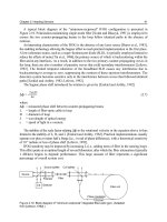
Figure 12.1 shows a mammogram as it might be interpreted according to current paradigms—these are not actual interpretations, just schematics to illustrate essential differences
between the paradigms. The arrows point to two real lesions (as determined by subsequent
follow-up of the patient) and the three lightly shaded crosses indicate perceived lesions or
suspicious regions. From now on, for brevity, the author will use the term suspicious region.

The numbers and locations of suspicious regions depend on the case and the observer’s skill
level. Some images are so obviously non-diseased that the radiologist sees nothing suspicious in
them, or they are so obviously diseased that the suspicious regions are conspicuous. Then there is
the gray area where one radiologist’s suspicious region may not correspond to another radiologist’s
suspicious region.
In Figure 12.1, evidently the radiologist found one of the lesions (the lightly shaded cross near the
left-most arrow), missed the other one (pointed to by the second arrow), and mistook two normal
structures for lesions (the two lightly shaded crosses that are relatively far from the true lesions).
To repeat, the term lesion is always a true or real lesion. The prefix true or real is implicit. The term
suspicious region is reserved for any region that, as far as the observer is concerned, has lesion-like
characteristics, but may not be a true lesion.
1. In the ROC paradigm, Figure 12.1 (top left), the radiologist assigns a single rating indicating the confidence level that there is at least one lesion somewhere in the image.* Assuming
a 1 through 5 positive directed integer rating scale, if the left-most lightly shaded cross is a
highly suspicious region then the ROC rating might be 5 (highest confidence for presence of
disease).
2. In the FROC paradigm, Figure 12.1 (top right), the dark shaded crosses indicate suspicious
regions that were marked or reported in the clinical report, and the adjacent numbers are the
corresponding ratings, which apply to specific regions in the image, unlike ROC, where the
rating applies to the whole image. Assuming the allowed positive-directed FROC ratings
are 1 through 4, two marks are shown, one rated FROC-4, which is close to a true lesion,
and the other rated FROC-1, which is not close to any true lesion. The third suspicious
region, indicated by the lightly shaded cross, was not marked, implying its confidence level
did not exceed the lowest reporting threshold. The marked region rated FROC-4 (highest
FROC confidence) is likely what caused the radiologist to assign the ROC-5 rating to this
image in the top-left figure. (For clarity the rating is specified alongside the applicable
paradigm.)
3. In the LROC paradigm, Figure 12.1 (bottom-left), the radiologist provides a rating summarizing confidence that there is at least one lesion somewhere in the image (as in the ROC paradigm) and marks the most suspicious region in the image. In this example, the rating might
be LROC-5, the 5 rating being the same as in the ROC paradigm, and the mark may be the
suspicious region rated FROC-4 in the FROC paradigm, and, since it is close to a true lesion,
in LROC terminology it would be recorded as a correct localization. If the mark were not near

a lesion it would be recorded as an incorrect localization. Only one mark is allowed in this
paradigm, and in fact one mark is required on every image, even if the observer does not find
* The author’s imaging physics mentor, Prof. Gary T. Barnes, had a way of emphasizing the word “somewhere” when he
spoke about the neglect of localization in ROC methodology, as in, “what do you mean the lesion is somewhere in the
image? If you can see it you should point to it.” Some of his grant applications were turned down because they did not
include ROC studies, yet he was deeply suspicious of the ROC method because it neglected localization information.
Around 1983 he guided the author toward a publication by Bunch et al., to be discussed in Section 12.4 and that started
the author’s career in this field.


262 The FROC paradigm

any suspicious region to report. The forced mark has caused confusion in the interpretation of
this paradigm and its usage. The late Prof. “Dick” Swensson has been the prime contributor to
this paradigm.
4. In the ROI paradigm, the researcher segments the image into a number of ROIs and the radiologist rates each ROI for presence of at least one suspicious region somewhere within the ROI.
The rating is similar to the ROC rating, except it applies to the segmented ROI, not the whole
image. Assuming a 1 through 5 positive-directed integer rating scale, in Figure 12.1 (bottomright) there are four ROIs and the ROI at ~9 o’clock might be rated ROI-5 as it contains the
most suspicious light cross, the one at ~11 o’clock might be rated ROI-1 as it does not contain
any light crosses, the one at ~3 o’clock might be rated ROI-2 or 3 (the light crosses would
tend to increase the confidence level), and the one at ~7 o’clock might be rated ROI-1. When
different views of the same patient anatomy are available, it is assumed that all images are
segmented consistently, and the rating for each ROI takes into account all views of that ROI
in the different views. In the example shown in Figure 12.1 (bottom-right), each case yields
four ratings. The segmentation shown in the figure is a schematic. In fact, the ROIs could be
clinically driven descriptors of location, such as apex of lung or mediastinum, and the image
does not have to have lines showing the ROIs (which would be distracting to the radiologist).
The number of ROIs per image can be at the researcher’s discretion and there is no requirement that every case have a fixed number of ROIs. Prof. Obuchowski has been the principal
contributor to this paradigm.
The rest of the book focuses on the FROC paradigm. It is the most general paradigm, special

cases of which accommodate other paradigms. As an example, for diffuse interstitial lung disease,
clearly a candidate for the ROC paradigm, the radiologist is implicitly pointing to the lung when
disease is seen.

ROC

FROC

4
1

LROC

ROI

Figure 12.1 A mammogram interpreted according to current observer performance paradigms. The
arrows indicate two real lesions and the three light crosses indicate suspicious regions. Evidently
the radiologist saw one of the lesions, missed the other lesion, and mistook two normal structures
for lesions. ROC (top-left): the radiologist assigns a single confidence level that somewhere in the
image there is at least one lesion. FROC (top-right): the dark crosses indicate suspicious regions that
are marked and the accompanying numerals are the FROC ratings. LROC (bottom-left): the radiologist provides a single rating that somewhere in the image there is at least one lesion and marks the
most suspicious region. ROI (bottom-right): the image is divided into a number of regions of interest
(by the researcher) and the radiologist rates each ROI for presence of at least one lesion somewhere
within the ROI.


12.3 The FROC paradigm as a search task 263

12.3 The FROC paradigm as a search task
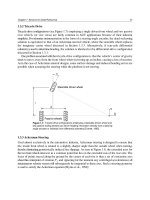
The FROC paradigm is equivalent to a search task. Any search task has two components: (1) finding

something and (2) acting on it. An example of a search task is looking for lost car keys or a milk carton in the refrigerator. Success in a search task is finding the object. Acting on it could be driving to
work or drinking milk from the carton. There is search-expertise associated with any search task.
Husbands are notoriously bad at finding the milk carton in the refrigerator (the author owes this
analogy to Dr. Elizabeth Krupinski). Like anything else, search expertise is honed by experience,
that is, lots of practice. While the author is not good at finding the milk carton in the refrigerator,
he is good at finding files in his computer.
Likewise, a medical imaging search task has two components (1) finding suspicious regions and
(2) acting on each finding (finding, used as a noun, is the actual term used by clinicians in their
reports), that is, determining the relevance of each finding to the health of the patient, and whether
to report it in the official clinical report. A general feature of a medical imaging search task is that
the radiologist does not know a priori whether the patient is diseased and, if diseased, how many
lesions are present. In the breast-screening context, it is known a priori that about five out of 1000
cases have cancers, so 99.5% of the time, odds are that the case has no malignant lesions (the probability of finding benign suspicious regions is much higher,19 about 13% for women aged 40–45).
The radiologist searches the images for lesions. If a suspicious region is found, and provided it is
sufficiently suspicious, the relevant location is marked and rated for confidence in being a lesion.
The process is repeated for each suspicious region found in the case. A radiology report consists of
a listing of search-related actions specific to each patient. To summarize:
Free-response data = variable number (≥0) of mark-rating pairs per case. It is a record of the
search process involved in finding disease and acting on each finding.

12.3.1 Proximity criterion and scoring the data
In the first two clinical applications of the FROC paradigm,9,20 the marks and ratings were indicated by a grease pencil on an acrylic overlay aligned, in a reproducible way, to the CRT displayed
chest image. Credit for a correct detection and localization, termed a lesion-localization or LLevent,* was given only if a mark was sufficiently close to an actual diseased region. Otherwise, the
observer’s mark-rating pair was scored as a non-lesion localization or NL-event.

The use of ROC terminology, such as true positives or false positives to describe FROC data,
seen in the literature on this subject, including the author’s earlier papers6, is not conducive to
clarity, and is strongly discouraged.

The classification of each mark as either an LL or an NL is referred to as scoring the marks.

Definition:
NL = non-lesion localization, that is, a mark that is not close to any lesion.
LL = lesion localization, that is, a mark that is close to a lesion.

* The proper terminology for this paradigm has evolved. Older publications and some newer ones refer to these as true
positive (TP) event, thereby confusing a ROC-related term that does not involve search with one that does.


264 The FROC paradigm

What is meant by sufficiently close? One adopts an acceptance radius (for spherical lesions) or
proximity criterion (the more general case). What constitutes close enough is a clinical decision,
the answer to which depends on the application.21–23 This source of arbitrariness in the FROC paradigm, which has been used to question its usage,24 is more in the mind of some researchers than
in the clinic. It is not necessary for two radiologists to point to the same pixel in order for them to
agree that they are seeing the same suspicious region. Likewise, two physicians (e.g., the radiologist
finding the lesion on an x-ray and the surgeon responsible for resecting it) do not have to agree on
the exact center of a lesion in order to appropriately assess and treat it. More often than not, clinical
common sense can be used to determine whether a mark actually localized the real lesion. When
in doubt, the researcher should ask an independent radiologist (i.e., not one of the participating
readers) how to score ambiguous marks.
For roughly spherical nodules a simple rule can be used. If a circular lesion is 10 mm in diameter,
one can use the touching-coins analogy to determine the criterion for a mark to be classified as lesion
localization. Each coin is 10 mm in diameter, so if they touch, their centers are separated by 10 mm,
and the rule is to classify any mark within 10 mm of an actual lesion center as an LL mark, and if
the separation is greater, the mark is classified as an NL mark. A recent paper25 using FROC analysis
gives more details on appropriate proximity criteria in the clinical context. Generally, the proximity
criterion is more stringent for smaller lesions than for larger ones. However, for very small lesions
allowance is made so that the criterion does not penalize the radiologist for normal marking jitter.
For 3D images, the proximity criteria is different in the x-y plane versus the slice thickness axis.

For clinical datasets, a rigid definition of the proximity criterion should not be used; deference
should be paid to the judgment of an independent expert.

12.3.2 Multiple marks in the same vicinity
Multiple marks near the same vicinity are rarely encountered with radiologists, especially if the
perceived lesion is mass-like (the exception would be if the perceived lesions were speck-like objects
in a mammogram, and even here radiologists tend to broadly outline the region containing perceived specks—in the author’s experience they do not spend their valuable clinical time marking
individual specks with great precision). However, algorithmic readers, such as a CAD algorithm,
are not radiologists and do tend to find multiple regions in the same area. Therefore, algorithm
designers generally incorporate a clustering step26 to reduce overlapping regions to a single region
and assign to it the highest rating (i.e., the rating of the highest rated mark, not the rating of the
closest mark). The reason for using the highest rating is that this gives full and deserved credit for
the localization. Other marks in the same vicinity with lower ratings need to be discarded from
the analysis. Specifically, they should not be classified as NLs, because each mark has successfully
located the true lesion to within the clinically acceptable criterion, that is, any one of them is a good
decision because it would result in a patient recall and point further diagnostics.

12.3.3 Historical context
The term free-response was coined in 1961 by Egan et al.7 to describe a task involving the detection of brief audio tone(s) against a background of white-noise (white-noise is what one hears if an
FM tuner is set to an unused frequency). The tone(s) could occur at any instant within an active
listening interval, defined by an indicator light bulb that is turned on. The listener’s task was to
respond by pressing a button at the specific instant(s) when a tone(s) was perceived (heard). The
listener was uncertain how many true tones could occur in an active listening interval and when
they might occur. Therefore, the number of responses (button presses) per active interval was a
priori unpredictable: it could be zero, one, or more. The Egan et al. study did not require the listener to rate each button press, but apart from this difference and with a two-dimensional image
replacing the one-dimensional listening interval, the acoustic signal detection study is similar to


12.4 A pioneering FROC study in medical imaging 265

a common task in medical imaging, namely, prior to interpreting a screening case for possible
breast cancer, the radiologist does not know how many diseased regions are actually present and,
if present, where they are located. Consequently, the case (all four views and possibly prior images)
is searched for regions that appear to be suspicious for cancer. If one or more suspicious regions are
found, and the level of suspicion of at least one of them exceeds the radiologists’ minimum reporting threshold, the radiologist reports the region(s). At the author’s former institution (University
of Pittsburgh, Department of Radiology) the radiologists digitally outline and annotate (describe)
suspicious region(s) that are found. As one would expect from the low prevalence of breast cancer,
in the screening context United States, and assuming expert-level radiologist interpretations, about
90% of breast cases do not generate any marks, implying case-level specificity of 90%. About 10%
of cases generate one or more marks and are recalled for further comprehensive imaging (termed
diagnostic workup). Of marked cases about 90% generate one mark, about 10% generate two marks,
and a rare case generates three or more marks. Conceptually, a mammography screening report
consists of the locations of regions that exceed the threshold and the corresponding levels of suspicion, reported as a Breast Imaging Reporting and Data System (BI-RADS) rating.27,28 This type of
information defines the free-response paradigm as it applies to breast screening. Free-response is
a clinical paradigm. It is a misconception that the paradigm forces the observer to keep marking and
rating many suspicious regions per case—as the mammography example shows, this is not the case.
The very name of the paradigm, free-response, implies, in plain English, no forcing.
Described next is the first medical imaging application of this paradigm.

12.4 A pioneering FROC study in medical imaging
This section details a FROC paradigm phantom study with x-ray images conducted in 1978 that
is often overlooked. With the obvious substitution of clinical images for the phantom images, this
study is a template for how a FROC experiment should ideally be conducted. A detailed description
of it is provided to set up the paradigm, the terminology used to describe it, and concludes with the
FROC plot, which is still widely (and incorrectly, see Chapter 17) used as the basis for summarizing
performance in this paradigm.

12.4.1 Image preparation
Bunch et al.3 conducted a free-response paradigm study using simulated lesions. They drilled 10–20
small holes (the simulated lesions) at random locations in ten 5 cm x 5 cm x 1.6 mm Teflon™ sheets.

A Lucite™ plastic block 5 cm thick was placed on top of each Teflon™ sheet to decrease contrast and
increase scatter, thereby appropriately reducing visibility of the holes (otherwise the hole detection
task would be too easy; as in ROC, it is important that the task not be too easy or too difficult).
Imaging conditions (kVp, mAs) were chosen such that, in preliminary studies, approximately 50%
of the simulated lesions were correctly located at the observer’s lowest confidence level. To minimize memory effects, the sheets were rotated, flipped or replaced between exposures. Six radiographs of four adjacent Teflon sheets, arranged in a 10 cm x 10 cm square, were obtained. Of these
six radiographs, one was used for training purposes and the remaining five for data collection.
Contact radiographs (i.e., with high visibility of the simulated lesions, similar in concept to the
insert images of computerized analysis of mammography phantom images [CAMPI] described in
Section 11.12 and Online Appendix 12.B; the cited online appendix provides a detailed description
of the calculation of SNR in CAMPI) of the sheets were obtained to establish the true lesion locations. Observers were told that each sheet contained from zero to 30 simulated lesions. A mark had
to be within about 1 mm to count as a correct localization; a rigid definition was deemed unnecessary
(the emphasis is because this simple and practical advice is ignored, not by the user community, but
by ROC methodology experts). Once images had been prepared, observers interpreted them. The
following is how Bunch et al. conducted the image interpretation part of their experiment.


266 The FROC paradigm

12.4.2 Image interpretation and the 1-rating
Observers viewed each film and marked and rated any visible holes with a felt-tip pen on a transparent overlay taped to the film at one edge (this allowed the observer to view the film directly without
the distracting effect of previously made marks—in digital interfaces it is important to implement
a show/hide feature in the user interface).
The observers used a 4-point ordered rating scale with 4 representing most likely a simulated
lesion to 1 representing least likely a simulated lesion. Note the meaning of the 1-rating: least likely
a simulated lesion. There is confusion with some using the FROC-1 rating to mean definitely not a
lesion. If that were the observer’s understanding, then logically the observer would fill up the entire
image, especially parts outside the patient anatomy, with 1s, as each of these regions is definitely not
a lesion. Since the observer did not behave in this unreasonable way, the meaning of the FROC-1
rating, as they interpreted it, or were told, must have been: I am done with this image, I have nothing
more to report on this image, show me the next one.

When correctly used, the 1-rating means there is some finite, small, probability that the marked
region is a lesion. In this sense, the free-response rating scale is asymmetric. Compare the 5-rating ROC scale, where ROC-1 = patient is definitely not diseased and ROC-5 = patient is definitely
diseased. This is a symmetric confidence level scale. In contrast, the free-response confidence level
scale labels different degrees of positivity in presence of disease. Table 12.1 compares the ROC 5-rating study to a FROC 4-rating study.
The FROC rating is one less than the corresponding ROC rating because the ROC-1 rating is not used
by the observer; the observer indicates such images by the simple expedient of not marking them.

12.4.3 Scoring the data
Scoring the data was defined (Section 12.3.1) as the process of classifying each mark-rating pair
as NL or LL, that is, as an incorrect or a correct decision, respectively. In the Bunch et al. study,
after each case was read the person running the study (i.e., Phil Bunch) compared the marks on
the overlay to the true lesion locations on the contact radiographs and scored the marks as lesion
localizations (LLs: lesions correctly localized to within about 1 mm radius) or non-lesion localizations (NLs: all other marks). Bunch et al. actually used the terms true positive and false positive
to describe these events. This practice, still used in publications in this field, is confusing because
there is ambiguity about whether these terms, commonly used in the ROC paradigm, are being
applied to the case as a whole or to specific regions in the case.

Table 12.1 Comparison of ROC and FROC rating scales: Note the FROC rating is one less than the
corresponding ROC rating and that there is no rating corresponding to ROC-1. The observer’s way of
indicating definitely non-diseased images is by simply not marking them.
ROC paradigm

FROC paradigm
Observer’s
categorization

Rating

Observer’s
categorization

1

Definitely not-diseased

NA

Image is not marked

2

…

1

Just possible it is a lesion

3

2

…

4

3

Rating

5

Note: NA = not available.

Definitely diseased

4

Definitely a lesion


12.4 A pioneering FROC study in medical imaging 267

12.4.4 The free-response receiver operating
characteristic (FROC) plot
The free-response receiver operating characteristic (FROC) plot was introduced, also in an auditory detection task, by Miller29 as a way of visualizing performance in the free-response auditory
tone detection task. In the medical imaging context, assume the marks have been classified as NLs
(non-lesion localizations) or LLs (lesion localizations), along with their associated ratings. Nonlesion localization fraction (NLF) is defined as the total number of NLs at or above a threshold
rating divided by the total number of cases. Lesion localization fraction (LLF) is defined as the
total number of LLs at or above the same threshold rating divided by the total number of lesions.
The FROC plot is defined as that of LLF (ordinate) versus NLF, as the threshold is varied. While
the ordinate LLF is a proper fraction, for example, 30/40 assuming 30 LLs and 40 true lesions, the
abscissa is an improper fraction that can exceed unity, for example, 35/21 assuming 35 NLs on 21
cases. The NLF notation is not ideal; it is used for notational symmetry and compactness.

Definitions:
• NLF = cumulated NL counts at or above threshold rating divided by total number of
cases.
• LLF = cumulated LL counts at or above threshold rating divided by total number of
lesions.
• The FROC curve is the plot of LLF (ordinate) versus NLF.
• The upper-right most operating point is termed the end-point and its coordinates are

denoted ( NLFmax , LLFmax ) .

Following Miller’s suggestion, Bunch et al.8,30 plotted lesion localization fraction (LLF) along
the ordinate versus non-lesion localization fraction (NLF) along the abscissa. Corresponding to
the different threshold ratings, pairs of (NLF, LLF) values, or operating points on the FROC, were
plotted. For example, in a positive directed 4-rating FROC study, such as employed by Bunch
et al., four FROC operating points result: those corresponding to marks rated 4s; those corresponding to marks rated 4s or 3s; the 4s, 3s, or 2s; and finally, the 4s, 3s, 2s, or 1s. An R-rating
(integer R > 0) FROC study yields at most R operating points. So, Bunch et al. were able to plot
only four operating points per reader, Figure 6 in Ref. 8.* Lacking a method of fitting a continuous FROC curve to the operating points, they did the best they could, and manually Frenchcurved fitted curves. In 1986, the author followed the same practice in his first paper on this
topic.9 In 1989 the author described6 a method for fitting such operating points, and developed
software called FROCFIT, but the fitting method is obsolete as the underlying statistical model
has been superseded; see Chapter 16. Moreover, it is now known, see Chapter 17, that the FROC
plot is a poor visual descriptor of performance.
If continuous ratings are used, the procedure is to start with a high threshold so none of
the ratings exceed the threshold, and gradually lower the threshold. Every time the threshold
crosses the rating of a mark, or possibly multiple marks, the total count of LLs and NLs exceeding the threshold is divided by the appropriate denominators yielding the raw FROC plot.
For example, when an LL rating just exceeds the threshold, the operating point jumps up by
* Figure 7 ibid has about 12 operating points as it includes three separate interpretations by the same observer. Moreover,
the area scaling implicit in the paper assumes a homogenous and isotropic image, that is, the probability of a NL is
proportional to the image area over which it is calculated, which is valid for a uniform background phantom. Clinical
images are not homogenous and isotropic and therefore not scalable in the Bunch et al. sense.


268 The FROC paradigm

1/(total number of lesions), and if two LLs simultaneously just exceed the threshold, the operating point jumps up by 2/(total number of lesions). If an NL rating just exceeds the threshold,
the operating point jumps to the right by 1/(total number of cases). If an LL rating and an NL
rating simultaneously just exceed the threshold, the operating point moves diagonally, up by
1/(total number of lesions) and to the right by 1/(total number of cases). The reader should
get the general idea by now and recognize that the cumulating procedure is very similar to

the manner in which ROC operating points were calculated, the only differences being in the
quantities being cumulated and the relevant denominators.
Having seen how a binned data FROC study is conducted and scored, and the results Frenchcurved as a FROC plot, typical simulated plots, generated under controlled conditions, are shown
next, both for continuous ratings data and for binned rating data. Such demonstrations, illustrating
trends, are impossible using real datasets. The reader should take the author’s word for it (for now)
that the simulator used is the simplest one possible that incorporates key elements of the search
process. Details of the simulator are given in Chapter 16, but for now the following summary
should suffice.

The simulator is characterized by three parameters μ, λ, and ν. The ν parameter characterizes the ability of the observer to find lesions. The λ parameter characterizes the ability of
the observer to avoid finding non-lesions. The μ parameter characterizes the ability of the
observer to correctly classify a found suspicious region as a true lesion or a non-lesion. The
reader should think of μ as a perceptual signal-to-noise ratio (pSNR) or conspicuity of
the lesion, similar to the separation parameter of the binormal model, that separates two
normal distributions describing the sampling of ratings of NLs and LLs. The simulator
also needs to know the number of lesions per diseased case, as this determines the number
of possible LLs on each case. Finally, there is a threshold parameter ζ1 that determines
whether a found suspicious region is actually marked. If ζ1 is negative infinity, then all
found suspicious regions are marked and conversely, as ζ1 increases, only those suspicious
regions whose confidence levels exceed ζ1 are marked. The concept of pSNR is clarified in
Section 12.5.2.

12.5 Population and binned FROC plots
Figure 12.2a through c shows simulated population FROC plots when the ratings are not binned,
generated by file mainFrocCurvePop.R described in Appendix 12.A. FROC data from 20,000
cases, half of them non-diseased, are generated (the code takes a while to finish). The very large
number of cases minimizes sampling variability, hence the term, population curves. Additionally,
the reporting threshold ζ1 was set to negative infinity to ensure that all suspicious regions are
marked. With higher thresholds, suspicious regions with confidence levels below the threshold
would not be marked and the rightward and upward traverses of the curves would be truncated.

Plots in Figure 12.2a through c correspond to μ equal to 0.5, 1, and 2, respectively. Plots in Figure
12.2d through f correspond to 5-rating binned data for 50 non-diseased and 50 diseased cases, and
the same values of μ; the relevant file is mainFrocCurveBinned.R.
1. Plots in Figure 12.2a through c show quasi-continuous plots while Figure 12.2 d through f show
operating points, five per plot, connected by straight line segments, so they are termed empirical FROC curves, analogous to the empirical ROC curves encountered in previous chapters. At


12.5 Population and binned FROC plots 269

a microscopic level plots (a) through (c) are also discrete, but one would need to zoom in to see
the discrete behavior (upward and rightward jumps) as each rating crosses a sliding threshold.
2. The empirical plots in the bottom row (d) through (f) of Figure 12.2 are subject to sampling
variability and will not, in general, match the population plots. The reader should try different
values of the seed variable in the code.
3. In general, FROC plots do not extend indefinitely to the right. Figure 5 in the Bunch et al.
paper is incorrect in implying, with the arrows, that the plots extend indefinitely to the right.
(Notation differences: In Bunch et al., P(TP) or v is equivalent to the author’s LLF. The variable Bunch et al. call λ is equivalent to NLF in this book.)
4. Like a ROC plot, the population FROC curve rises monotonically from the origin, initially
with infinite slope (this may not be evident for Figure 12.2a, but it is true; see code snippet
12.5.1). If all suspicious regions are marked, that is, ζ1 = −∞ , the plot reaches its upper rightmost limit, termed the end-point, with zero slope (again, this may not be evident for (a), but it
is true [see code snippet below]; here x and y are arrays containing NLF and LLF, respectively).
In general, these characteristics, that is, initial infinite slope and zero final slope, are not true
for empirical plots Figure 12.2d through f.

12.5.1 Code snippet

> mu
[1] 0.5
> (y[2]-y[1])/(x[2]-x[1]) # slope at origin
[1] Inf

> (y[10000]-y[10000-1])/(x[10000]-x[10000-1]) # slope at end-point
[1] 0

5. Assuming all suspicious regions are marked, the end-point (NLFmax , LLFmax ) represents a literal
end of the extent of the population FROC curve. This will become clearer in following chapters,
but for now it should suffice to note that the region of the population FROC plot to the upper right
of the end-point is inaccessible to the observer. [If sampling variability is taken into account it is
possible for the observed end-point to extend into this inaccessible space.]
6. There is an inverse correlation between LLFmax and NLFmax analogous to that between sensitivity and specificity in ROC analysis. The end-point (NLFmax , LLFmax ) of the FROC tends to
approach the point (0,1) as the perceptual SNR of the lesions approaches infinity. As μ decreases
the FROC curve approaches the x-axis and extends to large values along the abscissa, as in
Figure 12.2b. This is the chance-level FROC, where the reader detects few lesions, and makes
many NL marks.
7. The slope of the population FROC decreases monotonically as the operating point moves up
the curve, always staying non-negative, and it approaches zero, flattening out at an ordinate
less than unity. Some publications31 (Figure 3 ibid.) and Reference [32] (Figure 1 ibid.) incorrectly show LLF reaching unity. This is generally not the case unless the lesions are particularly conspicuous. This is well known to CAD researchers and to anyone who has conducted
FROC studies with radiologists. LLF reaches unity for large μ, which can be confirmed by
setting μ to a large value, for example, 10, Figure 12.3a. On the unit variance normal distribution scale, a value of 10, equivalent to 10 standard deviations, is effectively infinite.


0.75

1.00

0.00

0.25

0.50

0.75

1.0

0.0

0.4
NLF
(e)

0.50
NLF
(b)

0.2

0.25

0.6

0.75

0.8

1.00

0.50

0.75

1.00

0.0

0.0

0.1

0.1

NLF
(f )

0.2

0.2
NLF
(c)

0.3

0.3

0.4

0.4

0.5

Figure 12.2 Top row, (a) through (c): Population FROC plots for μ = 0.5, 1, 2; the other parameters are λ = 1, ν = 1, ζ1 = −∞ , and L max = 2 is the

maximum number of lesions per case in the dataset. The plots in the bottom row (d) through (f) correspond to 50 non-diseased and 70 diseased cases,
where the data was binned into five bins, and other parameters are unchanged. As μ increases, the uppermost point moves upwards and to the left.
The top row of images was produced by MainFrocCurvePop.R while the bottom row by mainFrocCurveBinned.R.

0.00

0.50

0.75

1.00

0.0

0.00

2.0

0.00

1.5

1.5

0.25

0.5
1.0
NLF
(d)

NLF
(a)

0.00

0.25

0.50

0.75

1.00

0.25

0.0

0.5

0.00

0.25

0.50

0.75

1.00

0.25

0.50

0.0

LLF
LLF

LLF

LLF

LLF
LLF

1.00

270 The FROC paradigm


1.00

1.00

0.75

0.75

LLF

LLF

12.5 Population and binned FROC plots 271

0.50

0.25

0.00
0.000

0.50

0.25

0.00
0.025

0.050
NLF
(a)

0.075

0.10

0

25

50
NLF
(b)

75

100

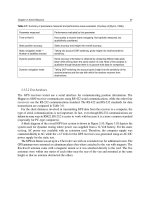
Figure 12.3 (a) FROC plot for μ = 10 in code file mainFrocCurvePop.R. Note the small range of the
NLF axis (it extends to 0.1). In this limit the ordinate reaches unity but the abscissa is limited to a small
value; see solar analogy Section 12.6 for explanation. (b) This plot corresponds to μ   = 0.01, depicting
near chance-level performance. Note the greatly increased traverse in the x-directions and the slight
upturn in the plot near NLF = 100.

12.5.2 Perceptual SNR
The shape and extent of the FROC plot is, to a large extent, determined by the perceptual* SNR of
the lesions, pSNR, modeled by parameter μ. Perceptual SNR is the ratio of perceptual signal to perceptual noise. To get to perceptual variables one needs a model of the eye-brain system that transforms physical image brightness variations to corresponding perceived brightness variations, and
such models exist.33–35 For uniform background images, like the phantom images used by Bunch
et al., a physical signal can be measured by a template function that has the same attenuation profile as the true lesion; an overview of this concept was given in Section 1.6. Assuming the template
is aligned with the lesion the cross-correlation between the template function and the image pixel
values is related to the numerator of SNR. The cross-correlation is defined as the summed product
of template function pixel values times the corresponding pixel values in the actual image. Next,
one calculates the cross-correlation between the template function and the pixel values in the
image when the template is centered over regions known to be lesion free. Subtracting the mean
of these values (over several lesion free regions) from the centered value gives the numerator of
SNR. The denominator is the standard deviation of the cross-correlation values in the lesion free
areas. Appendix 12.B has details on calculating physical SNR, which derives from the author’s
CAMPI (computer analysis of mammography phantom images) work 36–40. To calculate perceptual
SNR, one repeats these measurements but the visual process, or some model of it (e.g., the Sarnoff

JNDMetrix™ visual discrimination model35,41,42), is used to filter the image prior to calculation of
the cross-correlations.
An analogy may be helpful at this point. Finding the sun in the sky is a search task, so it can be
used to illustrate important concepts.

* Since humans make the decisions, it would be incorrect to label these as physical signal-to-noise ratios; that is the reason
for qualifying them as perceptual SNRs.


272 The FROC paradigm

12.6 The solar analogy: Search versus classification performance
Consider the sun, regarded as a lesion to be detected, with two daily observations spaced 12 hours
apart, so that at least one observation period is bound to have the sun somewhere up there. Furthermore,
the observer is assumed to know their GPS coordinates and have a watch that gives accurate local
time, from which an accurate location of the sun can be deduced. Assuming clear skies and no
obstructions to the view, the sun will always be correctly located and no reasonable observer will ever
generate a non-lesion localization or NL, that is, no region of the sky will be erroneously marked.
FROC curve implications of this analogy are as follows:
• Each 24-hour day corresponds to two trials in the Egan et al. sense,6 or two cases—one
diseased and one non-diseased—in the medical imaging context.
• The denominator for calculating LLF is the total number of AM days, and the denominator for calculating NLF is twice the total number of 24-hour days.
• Most important, LLFmax = 1 and NLFmax = 0.
In fact, even when the sun is not directly visible due to heavy cloud cover, since the actual location of the sun can be deduced from the local time and GPS coordinates, the rational observer
will still mark the correct location of the sun and not make any false sun localizations or nonlesion localizations, NLs, in the context of FROC terminology. Consequently, even in this example
LLFmax   = 1 and NLFmax = 0.
The conclusion is that in a task where a target is known to be present in the field of view and its
location is known, the observer will always reach LLFmax = 1 and NLFmax = 0 . Why are LLF and NLF
subscripted max? By randomly not marking the position of the sun even though it is visible, for
example, using a coin toss to decide whether or not to mark the sun, the observer can “walk down”

the y-axis of the FROC plot, reaching LLF = 0 and NLF = 0.* Alternatively, the observer uses a very
large threshold for reporting the sun, and as this threshold is lowered the operating point “walks
down” the curve. The reason for allowing the observer to walk down the vertical is simply to demonstrate that a continuous FROC curve from the origin to the highest point (0,1) can in fact be realized.
Now consider a fictitious otherwise earth-like planet where the sun can be at random positions,
rendering GPS coordinates and the local time useless. All one knows is that the sun is somewhere, in
the upper or lower hemispheres, subtended by the sky. If there are no clouds and consequently one
can see the sun clearly during daytime, a reasonable observer would still correctly locate the sun
while not marking the sky with any incorrect sightings, so LLFmax   = 1 and NLFmax = 0 . This is because,
in spite of the fact that the expected location is unknown, the high contrast sun is enough to trigger
the peripheral vision system, so that even if the observer did not start out looking in the correct direction, peripheral vision will drag the observer’s gaze to the correct location for foveal viewing.
The implication of this is that two fundamentally different mechanisms from that considered
in conventional observer performance methodology, namely search and lesion-classification,
are involved. Search describes the process of finding the lesion while not finding non-lesions.
Classification describes the process, once a possible sun location has been found, of recognizing that it is indeed the sun and marking it. Recall that search involves two steps: finding the
object of the search and acting on it. Search and lesion-classification performances quantify
the abilities of an observer to perform these steps.

* The logic is very similar to that used in Section 3.9.1 to describe how the ROC observer can “walk along” the chance
diagonal of the ROC curve.


12.6 The solar analogy: Search versus classification performance 273

Think of the eye as two cameras: a low-resolution camera (peripheral vision) with a wide fieldof-view, plus a high-resolution camera (foveal vision) with a narrow field-of-view. If one were
limited to viewing with the high-resolution camera one would spend so much time steering the
high-resolution narrow field-of-view camera from spot to spot that one would have a hard time
finding the desired stellar object. Having a single high-resolution narrow field-of-view would also
have negative evolutionary consequences as one would spend so much time scanning and processing the surroundings with the narrow field of view vision that one would miss dangers or
opportunities. Nature has equipped us with essentially two cameras. The first low-resolution camera is able to digest large areas of the surroundings and process it rapidly so that if danger (or
opportunity) is sensed, then the eye-brain system rapidly steers the second high-resolution camera to the location of the danger (or opportunity). This is nature’s way of optimally using the finite

resources of the eye-brain system. For a similar reason, astronomical telescopes come with a wide
field-of-view lower resolution spotter scope.

Since the large field-of-view low-resolution peripheral vision system has complementary
properties to the small field-of-view high-resolution foveal vision system, one expects an
inverse correlation between search and lesion-classification performances. Stated generally,
search involves two complementary processes: finding the suspicious regions and deciding
whether the found region is actually a lesion, and an inverse correlation between performance in the two tasks is expected, (see Chapter 19).

When cloud cover completely blocks the fictitious random-position sun there is no stimulus to
trigger the peripheral vision system to guide the fovea to the correct location. Lacking any stimulus,
the observer is reduced to guessing and is led to different conclusions depending upon the benefits
and costs involved. If, for example, the guessing observer earns a dollar for each LL and is fined a
dollar for each NL, then the observer will likely not make any marks as the chance of winning a dollar is much smaller than losing many dollars. For this observer LLFmax = 0 and NLFmax = 0, and the
operating point is “stuck” at the origin. If, on the other hand, the observer is told every LL is worth
a dollar and there is no penalty to NLs, then with no risk of losing, the observer will fill up the sky
with marks. In the second situation, the locations of the marks will lie on a grid determined by the
ratio of the 4π solid angle (subtended by the spherical sky) and the solid angle Ω subtended by the
sun. By marking every possible grid location, the observer is guaranteed to detect the sun and earn
a dollar irrespective of its random location and reach LLF = 1, but now the observer will generate
lots of non-lesion localizations, so maximum NLF will be large:
NLFmax =

4π
Ω

(12.1)

The FROC plot for this guessing observer is the straight line joining (0,0) to (NLFmax ,1) . For
example, if the observer fills up half the sky, then the operating point, averaged over many trials, is

(0.5 NLFmax ,0.5)

(12.2)

Radiologists do not guess—there is much riding on their decisions—so in the clinical situation,
if the lesion is not seen, the radiologist will not mark the image at random.
The analogy is not restricted to the sun, which one might argue is an almost infinite SNR object
and therefore atypical. As another example, consider finding stars or planets. In clear skies, if
one knows the constellations, herein lies the role of expertise, one can still locate bright stars and
planets like Venus or Jupiter. With fewer bright stars and/or obscuring clouds, there will be false


274 The FROC paradigm

sightings and the FROC plot could approach a flat horizontal line at ordinate equal to zero, but the
astronomer will not fill up the sky with false sightings of a desired star.
False sightings of objects in astronomy do occur. Finding a new astronomical object is a search
task, with two outcomes: correct localization (LL) or incorrect localization (NL). At the time of
writing there is a hunt for a new planet, possibly a gas giant,* that is much further away than even
the newly demoted Pluto. There is an astronomer in Australia† who is particularly good at finding
super novae (an exploding star; one has to be looking in the right region of the sky at the right time
to see the relatively brief explosion). His equipment is primitive by comparison to the huge telescope at Mt. Palomar, but his advantage is that he can rapidly point his 15 “telescope at a new region
of the sky and thereby cover a lot more sky in a given unit of time than is possible with the 200” Mt.
Palomar telescope. His search expertise is particularly good. Once correctly localized or pointed
to, the Mt. Palomar telescope will reveal a lot more detail about the object than is possible with the
smaller telescope, that is, it has high lesion-classification accuracy. In the medical imaging context
this detail (the shape of the lesion, its edge characteristics, presence of other abnormal features, etc.)
allows the radiologist to diagnose whether the lesion is malignant or benign. Once again one sees
that there should be an inverse correlation between search and lesion-classification performances.

Prof. Jeremy Wolfe of Harvard University is an expert in visual search and the interested reader
is referred to his many publications.43,44 As noted by him, rare items are often missed. To paraphrase
him, things that are not seen often are often not seen.45 So the problem faced by an astronomer looking for supernova events, a terminal security agency baggage inspector looking for explosives, and
the radiologist interpreting a screening mammogram for rare cancers, are similar at a fundamental
level: all of these are low prevalence search tasks.

12.7 Discussion/Summary
This chapter has introduced the FROC paradigm, the terminology used to describe it, and a common operating characteristic associated with it, namely the FROC. In the author’s experience this
paradigm is widely misunderstood. The following rules are intended to reduce the confusion:
■
■
■

■

■

■
■

Avoid using the term lesion-specific to describe location-specific paradigms.
Avoid using the term lesion when one means a suspicious region that may not be a true lesion.
Avoid using ROC-specific terms, such as true positive and false positive, that apply to the
whole case, to describe location-specific terms such as lesion and non-lesion localization, that
apply to localized regions of the image.
Avoid using the FROC-1 rating to mean in effect “I see no more signs of disease in this image, ”
when in fact it should be used as the lowest level of a reportable suspicious region. The former
usage amounts to “wasting” a confidence level.
Do not show FROC curves as reaching the unit ordinate, as this is the exception rather than
the rule.

Do not conceptualize FROC curves as extending to arbitrarily large values to the right.
Arbitrariness of the proximity criterion and multiple marks in the same region are not clinical constraints. Interactions with clinicians will allow selection of an appropriate proximity
criterion for the task at hand and the second problem (multiple marks in the same region) only
occurs with algorithmic observers and is readily fixed.

Additional points made in this chapter are: There is an inverse correlation between LLFmax and
NLFmax analogous to sensitivity and specificity in ROC analysis. The end-point (NLFmax , LLFmax ) of
the FROC curve tends to approach the point (0,1) as the perceptual SNR of the lesions approaches
* />† />

References 275

infinity. The solar analogy is highly relevant to understanding the search task. In search tasks, two
types of expertise are at work: search and lesion-classification performances, and an inverse correlation between them is expected.
Online Appendix 12.A describes, and explains in detail, the code used to generate the population
FROC curves shown in Figure 12.2a through c. Online Appendix 11.B details how one calculates
physical signal-to-noise ratio (SNR) for an object on a uniform noise background. This is useful in
understanding the concept of perceptual signal-to-noise ratio denoted μ. Online Appendix 12.C
is for those who wish to understand the Bunch et al. paper8 in more depth. This paper has certain transformations, sometimes referred to as the Bunch transforms, which relate a ROC plot to
a FROC plot and vise-versa. It is not a model of FROC data. The reason for including it is that this
important paper is much overlooked, and if the author does not write it, no one else will.
The FROC plot is the first proposed way of visually summarizing FROC data. The next chapter
deals with different empirical operating characteristics that can be defined from an FROC dataset.

References
1. Black WC. Anatomic extent of disease: A critical variable in reports of diagnostic accuracy.
Radiology. 2000;217(2):319–320.
2. Halpern SD, Karlawish JH, Berlin JA. The continuing unethical conduct of underpowered
clinical trials. JAMA. 2002;288(3):358–362.
3. Black WC, Dwyer AJ. Local versus global measures of accuracy: An important distinction for

diagnostic imaging. Med Decis Making. 1990;10(4):266–273.
4. Obuchowski NA, Mazzone PJ, Dachman AH. Bias, underestimation of risk, and loss of statistical power in patient-level analyses of lesion detection. Eur Radiol. 2010;20:584–594.
5. Alberdi E, Povyakalo AA, Strigini L, Ayton P, Given-Wilson R. CAD in mammography: Lesionlevel versus case-level analysis of the effects of prompts on human decisions. Int J Comput
Assist Radiol Surg. 2008;3(1):115–122.
6. Chakraborty DP. Maximum likelihood analysis of free-response receiver operating characteristic (FROC) data. Med Phys. 1989;16(4):561–568.
7. Egan JP, Greenburg GZ, Schulman AI. Operating characteristics, signal detectability and the
method of free-response. J Acoust Soc Am. 1961;33:993–1007.
8. Bunch PC, Hamilton JF, Sanderson GK, Simmons AH. A free-response approach to the measurement and characterization of radiographic-observer performance. J Appl Photogr Eng.
1978;4:166–171.
9. Chakraborty DP, Breatnach ES, Yester MV, Soto B, Barnes GT, Fraser RG. Digital and conventional chest imaging: A modified ROC study of observer performance using simulated
nodules. Radiology. 1986;158:35–39.
10. Chakraborty DP, Winter LHL. Free-response methodology: Alternate analysis and a new
observer-performance experiment. Radiology. 1990;174:873–881.
11. Chakraborty DP, Berbaum KS. Observer studies involving detection and localization:
Modeling, analysis and validation. Med Phys. 2004;31(8):2313–2330.
12. Starr SJ, Metz CE, Lusted LB, Goodenough DJ. Visual detection and localization of radiographic images. Radiology. 1975;116:533–538.
13. Starr SJ, Metz CE, Lusted LB. Comments on generalization of Receiver Operating
Characteristic analysis to detection and localization tasks. Phys Med Biol. 1977;22:376–379.
14. Swensson RG. Unified measurement of observer performance in detecting and localizing
target objects on images. Med Phys. 1996;23(10):1709–1725.
15. Judy PF, Swensson RG. Lesion detection and signal-to-noise ratio in CT images. Med Phys.
1981;8(1):13–23.
16. Swensson RG, Judy PF. Detection of noisy visual targets: Models for the effects of spatial
uncertainty and signal-to-noise ratio. Percept Psychophys. 1981;29(6):521–534.


276 The FROC paradigm

17. Obuchowski NA, Lieber ML, Powell KA. Data analysis for detection and localization of multiple abnormalities with application to mammography. Acad Radiol. 2000;7(7):516–525.
18. Rutter CM. Bootstrap estimation of diagnostic accuracy with patient-clustered data. Acad

Radiol. 2000;7(6):413–419.
19. Ernster VL. The epidemiology of benign breast disease. Epidemiol Rev. 1981;3(1):184–202.
20. Niklason LT, Hickey NM, Chakraborty DP, et al. Simulated pulmonary nodules: Detection
with dual-energy digital versus conventional radiography. Radiology. 1986;160:589–593.
21. Haygood TM, Ryan J, Brennan PC, et al. On the choice of acceptance radius in free-response
observer performance studies. BJR. 2012;86(1021): 42313554.
22. Chakraborty DP, Yoon HJ, Mello-Thoms C. Spatial localization accuracy of radiologists in
free-response studies: Inferring perceptual FROC curves from mark-rating data. Acad Radiol.
2007;14:4–18.
23. Kallergi M, Carney GM, Gaviria J. Evaluating the performance of detection algorithms in
digital mammography. Med Phys. 1999;26(2):267–275.
24. Gur D, Rockette HE. Performance assessment of diagnostic systems under the FROC
paradigm: Experimental, analytical, and results interpretation issues. Acad Radiol.
2008;15:1312–1315.
25. Dobbins JT III, McAdams HP, Sabol JM, et al. Multi-institutional evaluation of digital tomosynthesis, dual-energy radiography, and conventional chest radiography for the detection
and management of pulmonary nodules. Radiology. 2016;282(1):236–250.
26. Hartigan JA, Wong MA. Algorithm AS 136: A k-means clustering algorithm. J R Stat Soc Ser C
Appl Stat. 1979;28(1):100–108.
27. D’Orsi CJ, Bassett LW, Feig SA, et al. Illustrated Breast Imaging Reporting and Data System.
Reston, VA: American College of Radiology; 1998.
28. D’Orsi CJ, Bassetty LW, Berg WA. ACR BI-RADS-Mammography. 4th ed. Reston, VA: American
College of Radiology; 2003.
29. Miller H. The FROC curve: A representation of the observer’s performance for the method of
free-response. J Acoust Soc Am. 1969;46(6):1473–1476.
30. Bunch PC, Hamilton JF, Sanderson GK, Simmons AH. A free-response approach to the
measurement and characterization of radiographic-observer performance. Proc SPIE.
1977;127:124–135. Boston, MA.
31. Popescu LM. Model for the detection of signals in images with multiple suspicious locations. Med Phys. 2008;35(12):5565–5574.
32. Popescu LM. Nonparametric signal detectability evaluation using an exponential transformation of the FROC curve. Med Phys. 2011;38(10):5690–5702.
33. Van den Branden Lambrecht CJ, Verscheure O. Perceptual quality measure using a spatiotemporal model of the human visual system. SPIE Proceedings Volume 2668, Digital

Video Compression: Algorithms and Technologies. Event: Electronic Imaging: Science and
Technology, 1996, San Jose, CA; 1996. doi: 10.1117/12.235440.
34. Daly SJ. Visible differences predictor: An algorithm for the assessment of image fidelity.
Digital images and human vision 4 (1993): 124–125. SPIE/IS&T 1992 Symposium on Electronic
Imaging: Science and Technology; 1992; San Jose, CA.
35. Lubin J. A visual discrimination model for imaging system design and evaluation. In:
Peli E, ed. Vision Models for Target Detection and Recognition. Vol. 2, pp. 245–357. Singapore:
World Scientific; 1995.
36. Chakraborty DP, Sivarudrappa M, Roehrig H. Computerized measurement of mammographic display image quality. Paper presented at: Proc SPIE Medical Imaging 1999: Physics
of Medical Imaging; 1999; San Diego, CA.
37. Chakraborty DP, Fatouros PP. Application of computer analyis of mammography phantom
images (CAMPI) methodology to the comparison of two digital biopsy machines. Paper
presented at: Proc SPIE Medical Imaging 1998: Physics of Medical Imaging; 24 July 1998,
1998.


References 277

38. Chakraborty DP. Comparison of computer analysis of mammography phantom images
(CAMPI) with perceived image quality of phantom targets in the ACR phantom. Paper
presented at: Proc. SPIE Medical Imaging 1997: Image Perception; 26–27 February 1997;
Newport Beach, CA.
39. Chakraborty DP. Computer analysis of mammography phantom images (CAMPI). Proc SPIE
Med Imaging 1997 Phys Med Imaging. 1997;3032:292–299.
40. Chakraborty DP. Computer analysis of mammography phantom images (CAMPI): An application to the measurement of microcalcification image quality of directly acquired digital
images. Med Phys. 1997;24(8):1269–1277.
41. Siddiqui KM, Johnson JP, Reiner BI, Siegel EL. Discrete cosine transform JPEG compression
vs. 2D JPEG2000 compression: JNDmetrix visual discrimination model image quality analysis. Paper presented at: Medical Imaging; 2005. SPIE Proceedings Volume 5748, Medical
Imaging 2005: PACS and Imaging Informatics; doi: 10.1117/12.596146, San Diego, CA.
42. Chakraborty DP. An alternate method for using a visual discrimination model (VDM) to optimize softcopy display image quality. J Soc Inf Display 2006;14(10):921–926.

43. Wolfe JM. Guided search 2.0: A revised model of visual search. Psychonomic Bull Rev.
1994;1(2):202–238.
44. Wolfe JM. Visual search. In: Pashler H, ed. Attention. London: University College London
Press; 1998.
45. Wolfe JM, Horowitz TS, Kenner NM. Rare items often missed in visual searches. Nature.
2005;435(26):439.



13
Empirical operating characteristics
possible with FROC data

13.1 Introduction
Operating characteristics are visual depicters of performance. Quantities derived from operating
characteristics can serve as figures of merit (FOMs), that is, quantitative measures of performance.
For example, the area under an empirical ROC is a widely used FOM in receiver operating characteristic (ROC) analysis. This chapter defines empirical operating characteristics possible with
FROC data.
Here is the organization of this chapter. A distinction between latent* and actual marks is made
followed by a summary of free-response ROC (FROC) notation applicable to a single dataset where
modality and reader indices are not needed. This is a key table, which will be referred to in later
chapters. Following this, the chapter is organized into two main parts: formalism and examples.
The formalism sections, Sections 13.3 through 13.9, give formula for calculating different empirical
operating characteristics. While dry reading, it is essential to master, and the concepts are not that
difficult. The notation may appear dense because the FROC paradigm allows an a priori unknown
number of marks and ratings per case, but deeper inspection should convince the reader that the
apparent complexity is needed. When applied to the FROC plot the formalism is used to demonstrate an important fact, namely the semi-constrained property of the observed end-point, unlike the
constrained ROC end-point, whose upper limit is (1,1).
The second part, Sections 13.10 through 13.14, consists of coded examples of operating characteristics. Section 13.15 is devoted to clearing up confusion, in a clinical journal, about “location-level true
negatives,” traceable in large part to misapplication of ROC terminology to location-specific tasks.

Unlike other chapters, in this chapter most of the code is not relegated to online appendices. This
is because the concepts are most clearly demonstrated at the code level. The FROC data structure is
examined in some detail. Raw and binned FROC, AFROC and ROC plots are coded under controlled
conditions. Emphasized is the fact that unmarked non-diseased regions, confusingly termed “location level true negatives,” are unmeasurable events that should not be used in analysis. A simulated
algorithmic observer and a simulated expert radiologist are compared using both FROC and AFROC
curves, showing that the latter is preferable. The code for this is in an online appendix. The chapter
* In previous publications the author has termed these possible or potential NLs or LLs; going by the dictionary definition
of latent (that is, of a quality or state) existing but not yet developed or manifest, the present usage seems more appropriate. The latent mark should not be confused with the latency property of the decision variable, that is, the invariance of
operating points to arbitrary monotone increasing functions of the decision variable.

279


280 Empirical operating characteristics possible with FROC data

concludes with recommendations on which operating characteristics to use and which to avoid. In
particular, the alternative free-response operating characteristic (AFROC) has desirable properties
that make it the preferred way of summarizing performance. An interesting example is given where
AFROC-AUC = 0.5 can occur, and indicates better-than-chance level performance.
The starting point is the distinction between latent and actual marks and FROC notation.

13.2 Latent versus actual marks
From Chapter 12, FROC data consists of mark-rating pairs. Each mark indicates the location of
a region suspicious enough to warrant reporting and the rating is the associated confidence level.
A mark is recorded as lesion localization (LL) if it is sufficiently close to a true lesion according to
the adopted proximity criterion; otherwise, it is recorded as non-lesion localization (NL).

• To distinguish between perceived suspicious regions and regions that were actually
marked, it is necessary to introduce the distinction between latent marks and actual
marks. A latent mark is defined as a suspicious region, regardless of whether it was

marked. A latent mark becomes an actual mark if it is marked.
• A latent mark is a latent LL if it is close to a true lesion and otherwise it is a latent NL.
A non-diseased case can only have latent NLs. A diseased case can have latent NLs and
latent LLs.

13.2.1 FROC notation
Recall from Section 3.2, that the ROC paradigm requires the existence of a case-dependent decision variable (Z-sample) and a case-independent decision threshold ζ, and the rule that if z ≥ ζ the
case is diagnosed as diseased and otherwise the case is diagnosed as non-diseased as usual, upper
case Z vs. lower case z denotes the difference between a random variable and a realized value.
Analogously, FROC data requires the existence of a case and location-dependent Z-sample associated with each latent mark and a case-independent reporting threshold ζ and the rule that a latent
mark is marked if z ≥ ζ. One needs to account, in the notation, for case and locations dependences
of z and the distinction between case-level and location-level ground truth. For example, a diseased
case can have many localized regions that are non-diseased and a few diseased regions (the lesions).
Clear notation is vital to understanding this paradigm. FROC notation is summarized in
Table 13.1 and it is important to bookmark this table, as it will be needed to understand the subsequent development of this subject. For ease of referencing, the table is organized into three columns: the first column is the row number, the second column has the symbol(s), and the third
column has the meaning(s) of the symbol(s).
Row 1: The case-truth index t refers to the case (or patient), with t = 1 for non-diseased and
t = 2 for diseased cases.
Row 2: Two indices kt t (row 2) are needed to select case kt in truth-state t (recall the need for two
case-level indices in ROC analysis, Table 5.1).
Row 3 and 4: For a similar reason, two more indices ls s are needed to select latent mark ls in local
truth-state s, where s = 1 corresponds to a latent NL and s = 2 corresponds to a latent LL. One
can think of ls as indexing the locations of different latent marks with local truth-state s.
Row 5: The realized Z-sample for case kt t and latent NL mark l11 is denoted z kt tl1 1. Latent NL marks
are possible on non-diseased and diseased cases (i.e., both values of t are allowed). The range


13.2 Latent versus actual marks 281

Table 13.1 This table summarizes FROC notation. See Section 13.2.1 for details

Row #

Symbols

1

t

2

kt t ; kt = 1,2,..., Kt

3

s

4

ls s

5

z kttl11; z k2 2l2 2

6

ζ1

7

ζ r ; r = 1,2,..., RFROC

8

Nktt ≥ 0, NT

9

Meanings
Case-level truth-state: t = 1 for non-diseased and t = 2 for
diseased case

Mark-level truth-state: s = 1 for NL and s = 2 for LL marks
Latent mark ls in mark-level truth-state s
Z-sample for case kt t and latent mark l11; −∞ < z kttl11 < ∞ provided
l1 ≠ ∅; otherwise it is an unobservable event; Z-sample for case
k2 2 and latent mark l2 2; unmarked lesions are assigned negative
infinity ratings
Lowest reporting threshold; latent mark is marked only if
z kttls s ≥ ζ1

K2

Lk2 , LT =

Case kt in case-level truth-state t; Kt is the total number of cases
in truth-state t

∑L

k2

If ζ r ≤ z kttls s < ζ r +1 mark is assigned rating r; dummy thresholds
are ζ0 = −∞, and ζ Rfroc +1 = ∞;RFROC is the number of FROC bins
Numbers of latent NLs on case kt t ; NT is the total number of
marked NLs in the dataset
Number of lesions in diseased case k2 2; total number of lesions
in dataset

k2 =1

10

l1, l2

Indexing latent marks: l1 = {∅} ⊕ {1,2,..., Nktt };l2 = {1,2,..., Lk2}

of a Z-sample is −∞ < z kt tl1 1 < ∞, provided l1 ≠ ∅; otherwise, it is an unobservable event (see text
box below). The Z-sample of a latent LL is z k2 2l2 2. Unmarked lesions are assigned null set labels
and negative infinity ratings; this is the meaning of z k2 2l2 2 l2 = ∅ = −∞.
Row 6 and 7: A latent mark is actually marked if z kt tls s ≥ ζ1 , where ζ1 is the lowest reporting threshold adopted by the observer. Additional thresholds (ζ2 , ζ3 ,...) are needed to accommodate
greater than one FROC bins. If marked, a latent NL is recorded as an actual NL, and likewise if
marked, a latent LL is recorded as an actual LL.

(

)

• If not marked, a latent NL is an unobservable event: more on this in Section 13.15. This
is a major source of confusion among some researchers familiar with the ROC paradigm

who use the highly misleading term location-level true negative for unmarked latent NLs.
• In contrast, unmarked lesions are observable events—one knows (trivially) which lesions
were not marked. In the analyses, unmarked lesions are assigned −∞ ratings, guaranteed
to be smaller than any rating used by the observer.

Row 8: N kt t ≥ 0 is the total number of latent NL marks on case kt t . NT is the total number of latent
NLs in the dataset.
It is an a priori unknown modality-reader-case dependent non-negative random integer. It is
incorrect to estimate it by dividing the image area by the lesion area because not all regions
of the image are equally likely to have lesions, lesions do not have the same size, and most