Lecture note Computer Organization - Part 2.2: The computer system
Bạn đang xem bản rút gọn của tài liệu. Xem và tải ngay bản đầy đủ của tài liệu tại đây (1.21 MB, 194 trang )
CHAPTER
EXTERNAL MEMORY
6.1
Magnetic Disk
Magnetic Read and Write Mechanisms Data Organization
and Formatting Physical Characteristics
Disk Performance Parameters
6.2
Raid
RAID Level 0
RAID Level 1
RAID Level 2
RAID Level 3
RAID Level 4
RAID Level 5
RAID Level 6
6.3
Optical Memory
Compact Disk Digital Versatile Disk
HighDefinition Optical Disks
184
6.4
Magnetic Tape
6.5
Recommended Reading and Web Sites
6.6
Key Terms, Review Questions, and Problems
This chapter examines a range of external memory devices and systems. We begin
with the most important device, the magnetic disk. Magnetic disks are the
foundation of ex ternal memory on virtually all computer systems. The next
section examines the use of disk arrays to achieve greater performance, looking
specifically at the family of systems known as RAID (Redundant Array of
Independent Disks). An increasingly important component of many computer
systems is external optical memory, and this is examined in the third section.
Finally, magnetic tape is described.
6.1 MAGNETIC DISK
A disk is a circular platter constructed of nonmagnetic material, called the
substrate, coated with a magnetizable material. Traditionally, the substrate has
been an alu minum or aluminum alloy material. More recently, glass substrates
have been intro duced. The glass substrate has a number of benefits, including
the following:
• Improvement in the uniformity of the magnetic film surface to increase disk
reliability
• A significant reduction in overall surface defects to help reduce readwrite
errors
• Ability to support lower fly heights (described subsequently)
• Better stiffness to reduce disk dynamics
• Greater ability to withstand shock and damage
Magnetic Read and Write Mechanisms
Data are recorded on and later retrieved from the disk via a conducting coil named
the head; in many systems, there are two heads, a read head and a write head.
During a read or write operation, the head is stationary while the platter rotates
beneath it. The write mechanism exploits the fact that electricity flowing through
a coil produces a magnetic field. Electric pulses are sent to the write head, and the
resulting
Read
current
MR
sensor
Write current
Shield
Inductive
write element
Magnetization
Recording
medium
Figure 6.1 Inductive Write/Magnetoresistive Read
Head
magnetic patterns are recorded on the surface below, with different patterns for
pos itive and negative currents. The write head itself is made of easily
magnetizable ma terial and is in the shape of a rectangular doughnut with a gap
along one side and a few turns of conducting wire along the opposite side (Figure
6.1). An electric current in the wire induces a magnetic field across the gap,
which in turn magnetizes a small area of the recording medium. Reversing the
direction of the current reverses the di rection of the magnetization on the
recording medium.
The traditional read mechanism exploits the fact that a magnetic field
moving relative to a coil produces an electrical current in the coil. When the
surface of the disk passes under the head, it generates a current of the same
polarity as the one already recorded. The structure of the head for reading is in
this case essentially the same as for writing and therefore the same head can be
used for both. Such single heads are used in floppy disk systems and in older
rigid disk systems.
Contemporary rigid disk systems use a different read mechanism, requiring
a separate read head, positioned for convenience close to the write head. The read
head consists of a partially shielded magnetoresistive (MR) sensor. The MR
material has an electrical resistance that depends on the direction of the
magnetization of the medium moving under it. By passing a current through the
MR sensor, resistance changes are detected as voltage signals. The MR design
allows higherfrequency operation, which equates to greater storage densities and
operating speeds.
Data Organization and Formatting
The head is a relatively small device capable of reading from or writing to a
portion of the platter rotating beneath it. This gives rise to the organization of
data on the
Sectors
Tracks
Intersector gap
Intertrack gap
Figure 6.2 Disk Data Layout
platter in a concentric set of rings, called tracks. Each track is the same width as
the head. There are thousands of tracks per surface.
Figure 6.2 depicts this data layout. Adjacent tracks are separated by gaps.
This prevents, or at least minimizes, errors due to misalignment of the head or
simply interference of magnetic fields.
Data are transferred to and from the disk in sectors (Figure 6.2). There are
typically hundreds of sectors per track, and these may be of either fixed or
variable length. In most contemporary systems, fixedlength sectors are used,
with 512 bytes being the nearly universal sector size. To avoid imposing
unreasonable precision requirements on the system, adjacent sectors are separated
by intratrack (intersec tor) gaps.
A bit near the center of a rotating disk travels past a fixed point (such as a
read–write head) slower than a bit on the outside. Therefore, some way must be
found to compensate for the variation in speed so that the head can read all the
bits at the same rate. This can be done by increasing the spacing between bits of
informa tion recorded in segments of the disk. The information can then be
scanned at the same rate by rotating the disk at a fixed speed, known as the
constant angular veloc ity (CAV). Figure 6.3a shows the layout of a disk using
CAV. The disk is divided into a number of pieshaped sectors and into a series of
concentric tracks. The advantage of using CAV is that individual blocks of data
can be directly addressed by track and sector. To move the head from its current
location to a specific address, it only takes a short movement of the head to a
specific track and a short wait for the proper sec tor to spin under the head. The
disadvantage of CAV is that the amount of data that
(a) Constant angular velocity
(b) Multiple zoned recording
Figure 6.3 Comparison of Disk Layout Methods
can be stored on the long outer tracks is the only same as what can be stored on
the short inner tracks.
Because the density, in bits per linear inch, increases in moving from the
out ermost track to the innermost track, disk storage capacity in a
straightforward CAV system is limited by the maximum recording density that
can be achieved on the in nermost track. To increase density, modern hard disk
systems use a technique known as multiple zone recording, in which the surface
is divided into a number of concentric zones (16 is typical). Within a zone, the
number of bits per track is con stant. Zones farther from the center contain more
bits (more sectors) than zones closer to the center. This allows for greater overall
storage capacity at the expense of somewhat more complex circuitry. As the disk
head moves from one zone to an other, the length (along the track) of individual
bits changes, causing a change in the timing for reads and writes. Figure 6.3b
suggests the nature of multiple zone record ing; in this illustration, each zone is
only a single track wide.
Some means is needed to locate sector positions within a track. Clearly,
there must be some starting point on the track and a way of identifying the start
and end of each sector. These requirements are handled by means of control data
recorded on the disk. Thus, the disk is formatted with some extra data used only
by the disk drive and not accessible to the user.
An example of disk formatting is shown in Figure 6.4. In this case, each
track contains 30 fixedlength sectors of 600 bytes each. Each sector holds 512
bytes of data plus control information useful to the disk controller. The ID field is
a unique identifier or address used to locate a particular sector. The SYNCH byte
is a special bit pattern that delimits the beginning of the field. The track number
identifies a track on a surface. The head number identifies a head, because this
disk has multi ple surfaces (explained presently). The ID and data fields each
contain an error detecting code.
Physical Characteristics
Table 6.1 lists the major characteristics that differentiate among the various types
of magnetic disks. First, the head may either be fixed or movable with respect to
the ra dial direction of the platter. In a fixedhead disk, there is one readwrite
head per
Index
Gap 1
Bytes
17
7
Bytes 1
2
ID
Gap 2
field
41
515
1
1
Data
field
20
2
Gap
17
7
41
515
1
20
512
17
7
41
515
20
2
Figure 6.4 Winchester Disk Format (Seagate ST506)
track. All of the heads are mounted on a rigid arm that extends across all tracks;
such systems are rare today. In a movablehead disk, there is only one readwrite
head. Again, the head is mounted on an arm. Because the head must be able to be
positioned above any track, the arm can be extended or retracted for this purpose.
The disk itself is mounted in a disk drive, which consists of the arm, a
spindle that rotates the disk, and the electronics needed for input and output of
binary data. A nonremovable disk is permanently mounted in the disk drive; the
hard disk in a personal computer is a nonremovable disk. A removable disk can
be removed and replaced with another disk. The advantage of the latter type is
that unlimited amounts of data are available with a limited number of disk
systems. Furthermore, such a disk may be moved from one computer system to
another. Floppy disks and ZIP cartridge disks are examples of removable disks.
For most disks, the magnetizable coating is applied to both sides of the
platter, which is then referred to as double sided. Some less expensive disk
systems use singlesided disks.
Table 6.1 Physical Characteristics of Disk Systems
Read–write head (1 per surface) Direction of
arm motion
Surface 9
Platter
Surface 8
Surface 7
Surface 6
Surface 5
Surface 4
Surface 3
Surface 2
Surface 1
Surface 0
Spindle
Boom
Figure 6.5 Components of a Disk Drive
Some disk drives accommodate multiple platters stacked vertically a
fraction of an inch apart. Multiple arms are provided (Figure 6.5). Multiple–
platter disks em ploy a movable head, with one readwrite head per platter
surface. All of the heads are mechanically fixed so that all are at the same
distance from the center of the disk and move together. Thus, at any time, all of
the heads are positioned over tracks that are of equal distance from the center of
the disk. The set of all the tracks in the same relative position on the platter is
referred to as a cylinder. For example, all of the shaded tracks in Figure 6.6 are
part of one cylinder.
Finally, the head mechanism provides a classification of disks into three
types. Traditionally, the readwrite head has been positioned a fixed distance
above the
Figure 6.6 Tracks and Cylinders
platter, allowing an air gap. At the other extreme is a head mechanism that
actually comes into physical contact with the medium during a read or write
operation. This mechanism is used with the floppy disk, which is a small,
flexible platter and the least expensive type of disk.
To understand the third type of disk, we need to comment on the
relationship between data density and the size of the air gap. The head must
generate or sense an electromagnetic field of sufficient magnitude to write and
read properly. The narrower the head is, the closer it must be to the platter surface
to function. A nar rower head means narrower tracks and therefore greater data
density, which is de sirable. However, the closer the head is to the disk, the
greater the risk of error from impurities or imperfections. To push the technology
further, the Winchester disk was developed. Winchester heads are used in sealed
drive assemblies that are almost free of contaminants. They are designed to
operate closer to the disk’s sur face than conventional rigid disk heads, thus
allowing greater data density. The head is actually an aerodynamic foil that rests
lightly on the platter’s surface when the disk is motionless. The air pressure
generated by a spinning disk is enough to make the foil rise above the surface.
The resulting noncontact system can be engi neered to use narrower heads that
operate closer to the platter’s surface than con ventional rigid disk heads.1
Table 6.2 gives disk parameters for typical contemporary highperformance
disks.
Table 6.2 Typical Hard Disk Drive Parameters
Seagate
Barracuda
Seagate
Barracuda
Seagate
Barracuda
Highcapacity
server
1 TB
Highperformance
desktop
750 GB
Entrylevel
desktop
160 GB
120 GB
Handheld
devices
8 GB
Minimum tracktotrack
seek time
Average seek time
0.8 ms
0.3 ms
1.0 ms
—
1.0 ms
8.5 ms
3.6 ms
9.5 ms
12.5 ms
12 ms
Spindle speed
7200 rpm
7200 rpm
7200
5400 rpm
3600 rpm
Average rotational delay
4.16 ms
4.16 ms
4.17 ms
5.6 ms
8.33 ms
Maximum transfer rate
3 GB/s
300 MB/s
300 MB/s
150 MB/s
10 MB/s
Bytes per sector
512
512
512
512
512
Tracks per cylinder (num
ber of platter surfaces)
8
8
2
8
2
Application
Capacity
Hitachi
Micro
Laptop
1
As a matter of historical interest, the term Winchester was originally used by IBM as a code name for
the 3340 disk model prior to its announcement. The 3340 was a removable disk pack with the heads
sealed within the pack. The term is now applied to any sealedunit disk drive with aerodynamic head
design. The Winchester disk is commonly found built in to personal computers and workstations,
where it is referred to as a hard disk.
Wait for
device
Wait for
channel
Seek
Rotational
delay
Data
transfer
Device busy
Figure 6.7 Timing of a Disk I/O Transfer
Disk Performance Parameters
The actual details of disk I/O operation depend on the computer system, the
operat ing system, and the nature of the I/O channel and disk controller
hardware. A gen eral timing diagram of disk I/O transfer is shown in Figure 6.7.
When the disk drive is operating, the disk is rotating at constant speed. To
read or write, the head must be positioned at the desired track and at the
beginning of the desired sector on that track. Track selection involves moving the
head in a movable head system or electronically selecting one head on a fixed
head system. On a movable head system, the time it takes to position the head at
the track is known as seek time. In either case, once the track is selected, the disk
controller waits until the appropriate sector rotates to line up with the head. The
time it takes for the beginning of the sector to reach the head is known as
rotational delay, or rotational latency. The sum of the seek time, if any, and the
rotational delay equals the access time, which is the time it takes to get into
position to read or write. Once the head is in po sition, the read or write
operation is then performed as the sector moves under the head; this is the data
transfer portion of the operation; the time required for the transfer is the transfer
time.
In addition to the access time and transfer time, there are several queuing
delays normally associated with a disk I/O operation. When a process issues an
I/O request, it must first wait in a queue for the device to be available. At that
time, the device is assigned to the process. If the device shares a single I/O
channel or a set of I/O channels with other disk drives, then there may be an
additional wait for the channel to be available. At that point, the seek is
performed to begin disk access.
In some highend systems for servers, a technique known as rotational posi
tional sensing (RPS) is used. This works as follows: When the seek command has
been issued, the channel is released to handle other I/O operations. When the
seek is completed, the device determines when the data will rotate under the
head. As that sector approaches the head, the device tries to reestablish the
communication path back to the host. If either the control unit or the channel is
busy with another I/O, then the reconnection attempt fails and the device must
rotate one whole revo lution before it can attempt to reconnect, which is called
an RPS miss. This is an extra delay element that must be added to the timeline of
Figure 6.7.
SEEK TIME Seek time is the time required to move the disk arm to the required
track. It turns out that this is a difficult quantity to pin down. The seek time
consists of two key components: the initial startup time, and the time taken to
traverse the tracks that have to be crossed once the access arm is up to speed.
Unfortunately, the traversal time is not a linear function of the number of tracks,
but includes a settling
time (time after positioning the head over the target track until track
identification is confirmed).
Much improvement comes from smaller and lighter disk components. Some
years ago, a typical disk was 14 inches (36 cm) in diameter, whereas the most
com mon size today is 3.5 inches (8.9 cm), reducing the distance that the arm
has to travel. A typical average seek time on contemporary hard disks is under 10
ms.
ROTATIONAL DELAY Disks, other than floppy disks, rotate at speeds ranging
from 3600 rpm (for handheld devices such as digital cameras) up to, as of this
writing, 20,000 rpm; at this latter speed, there is one revolution per 3 ms. Thus,
on the aver age, the rotational delay will be 1.5 ms.
TRANSFER TIME The transfer time to or from the disk depends on the rotation
speed of the disk in the following fashion:
T = b
rN
where
T = transfer time
b = number of bytes to be transferred
N = number of bytes on a track
r = rotation speed, in revolutions per second
Thus the total average access time can be expressed as
1
Ta = Ts +
b
+
2r rN
where Ts is the average seek time. Note that on a zoned drive, the number of bytes
per track is variable, complicating the calculation. 2
A TIMING COMPARISON With the foregoing parameters defined, let us look at two
different I/O operations that illustrate the danger of relying on average values. Con
sider a disk with an advertised average seek time of 4 ms, rotation speed of 15,000 rpm,
and 512byte sectors with 500 sectors per track. Suppose that we wish to read a file
consisting of 2500 sectors for a total of 1.28 Mbytes. We would like to estimate the
total time for the transfer.
First, let us assume that the file is stored as compactly as possible on the disk.
That is, the file occupies all of the sectors on 5 adjacent tracks (5 tracks 500
sectors/ track = 2500 sectors). This is known as sequential organization. Now, the
time to read the first track is as follows:
Average seek
4
ms Average rotational delay 2
ms Read 500 sectors
4
ms
10 ms
2
Compare the two preceding equations to Equation (4.1).
Suppose that the remaining tracks can now be read with essentially no seek
time. That is, the I/O operation can keep up with the flow from the disk. Then, at
most, we need to deal with rotational delay for each succeeding track. Thus each
successive track is read in 2 + 4 = 6 ms. To read the entire file,
Total time = 10 + (4 * 6) = 34 ms = 0.034 seconds
Now let us calculate the time required to read the same data using random
access rather than sequential access; that is, accesses to the sectors are distributed
randomly over the disk. For each sector, we have
Average seek 4 ms
Rotational delay 2 ms
Read 1 sectors 0.008 ms
6.008 ms
Total time = 2500 * 6.008 = 15020 ms = 15.02 seconds
It is clear that the order in which sectors are read from the disk has a
tremen dous effect on I/O performance. In the case of file access in which
multiple sectors are read or written, we have some control over the way in which
sectors of data are deployed. However, even in the case of a file access, in a
multiprogramming environ ment, there will be I/O requests competing for the
same disk. Thus, it is worthwhile to examine ways in which the performance of
disk I/O can be improved over that achieved with purely random access to the
disk. This leads to a consideration of disk scheduling algorithms, which is the
province of the operating system and beyond the scope of this book (see
[STAL09] for a discussion).
RAID Simulator
6.2 RAID
As discussed earlier, the rate in improvement in secondary storage performance
has been considerably less than the rate for processors and main memory. This
mis match has made the disk storage system perhaps the main focus of concern
in im proving overall computer system performance.
As in other areas of computer performance, disk storage designers
recognize that if one component can only be pushed so far, additional gains in
performance are to be had by using multiple parallel components. In the case of
disk storage, this leads to the development of arrays of disks that operate
independently and in parallel. With multiple disks, separate I/O requests can be
handled in parallel, as long as the data required reside on separate disks.
Further, a single I/O request
can be executed in parallel if the block of data to be accessed is distributed across
multiple disks.
With the use of multiple disks, there is a wide variety of ways in which the
data can be organized and in which redundancy can be added to improve
reliability. This could make it difficult to develop database schemes that are
usable on a number of platforms and operating systems. Fortunately, industry has
agreed on a standardized scheme for multipledisk database design, known as
RAID (Redundant Array of Independent Disks). The RAID scheme consists of
seven levels,3 zero through six. These levels do not imply a hierarchical
relationship but designate different design architectures that share three common
characteristics:
1. RAID is a set of physical disk drives viewed by the operating system as a
sin gle logical drive.
2. Data are distributed across the physical drives of an array in a scheme known
as striping, described subsequently.
3. Redundant disk capacity is used to store parity information, which
guarantees data recoverability in case of a disk failure.
The details of the second and third characteristics differ for the different RAID
lev els. RAID 0 and RAID 1 do not support the third characteristic.
The term RAID was originally coined in a paper by a group of researchers at
the University of California at Berkeley [PATT88].4 The paper outlined various
RAID configurations and applications and introduced the definitions of the RAID
levels that are still used. The RAID strategy employs multiple disk drives and
dis tributes data in such a way as to enable simultaneous access to data from
multiple drives, thereby improving I/O performance and allowing easier
incremental in creases in capacity.
The unique contribution of the RAID proposal is to address effectively the
need for redundancy. Although allowing multiple heads and actuators to operate
simultaneously achieves higher I/O and transfer rates, the use of multiple devices
increases the probability of failure. To compensate for this decreased reliability,
RAID makes use of stored parity information that enables the recovery of data
lost due to a disk failure.
We now examine each of the RAID levels. Table 6.3 provides a rough guide
to the seven levels. In the table, I/O performance is shown both in terms of data
trans fer capacity, or ability to move data, and I/O request rate, or ability to
satisfy I/O re quests, since these RAID levels inherently perform differently
relative to these two
3
Additional levels have been defined by some researchers and some companies, but the seven levels
described in this section are the ones universally agreed on.
4
In that paper, the acronym RAID stood for Redundant Array of Inexpensive Disks. The term
inexpensive was used to contrast the small relatively inexpensive disks in the RAID array to the
alterna tive, a single large expensive disk (SLED). The SLED is essentially a thing of the past, with
similar disk technology being used for both RAID and nonRAID configurations. Accordingly, the
industry has adopted the term independent to emphasize that the RAID array creates significant
performance and reliability gains.
Table 6.3 RAID Levels
Category
Level
Description
Disks
Required
Data Availability
Lower than
single disk
Striping
0
Nonredundant
Mirroring
1
Mirrored
2
Redundant via Ham
ming code
N + m
3
Bitinterleaved parity
N + 1
Much higher than single
disk; comparable to
RAID 2, 4, or 5
4
Blockinterleaved
parity
N + 1
Much higher than single
disk; comparable to
RAID 2, 3, or 5
5
Blockinterleaved
distributed parity
N + 1
6
Blockinterleaved
dual distributed
parity
Much higher than single
disk; comparable to
RAID 2, 3, or 4
N + 2
N
2N
Parallel access
Independent
access
N = number of data disks; m proportional to log N
Higher than RAID 2,
3, 4, or 5; lower than
RAID 6
Much higher than single
disk; comparable to
RAID 3, 4, or 5
Highest of all listed
alternatives
Large I/O Data
Transfer Capacity
Very high
Small I/O
Request Rate
Very high for both read
and write
Highest of all listed
alternatives
Up to twice that of a
single disk for read;
similar to single disk
for write
Approximately twice
that of a single disk
Highest of all listed
alternatives
Approximately twice
that of a single disk
Higher than single disk
for read; similar to sin
gle disk for write
Similar to RAID 0 for
read; significantly lower
than single disk for
write
Similar to RAID 0 for
read; lower than single
disk for write
Similar to RAID 0 for
read; lower than RAID
5 for write
Similar to RAID 0 for
read; significantly lower
than single disk for
write
Similar to RAID 0 for
read; generally lower
than single disk for
write
Similar to RAID 0 for
read; significantly lower
than RAID 5 for write
(a)
RAID 0 (Nonredundant)
(b)
RAID 1 (Mirrored)
(c)
RAID 2 (Redundancy through Hamming code)
Figure 6.8 RAID Levels
metrics. Each RAID level’s strong point is highlighted by darker shading. Figure
6.8 illustrates the use of the seven RAID schemes to support a data capacity
requiring four disks with no redundancy. The figures highlight the layout of user
data and re dundant data and indicates the relative storage requirements of the
various levels. We refer to these figures throughout the following discussion.
RAID Level 0
RAID level 0 is not a true member of the RAID family because it does not
include redundancy to improve performance. However, there are a few
applications, such as some on supercomputers in which performance and capacity
are primary concerns and low cost is more important than improved reliability.
For RAID 0, the user and system data are distributed across all of the disks
in the array. This has a notable advantage over the use of a single large disk: If
two different I/O requests are pending for two different blocks of data, then there
is a good chance that the requested blocks are on different disks. Thus, the two
requests can be issued in parallel, reducing the I/O queuing time.
But RAID 0, as with all of the RAID levels, goes further than simply
distribut ing the data across a disk array: The data are striped across the
available disks. This is best understood by considering Figure 6.9. All of the user
and system data are viewed
(d)
RAID 3 (Bitinterleaved parity)
(e)
RAID 4 (Blocklevel parity)
(f)RAID 5 (Blocklevel distributed parity)
(g)
RAID 6 (Dual redundancy)
Figure 6.8 RAID Levels (continued )
as being stored on a logical disk. The logical disk is divided into strips; these
strips may be physical blocks, sectors, or some other unit. The strips are mapped
round robin to consecutive physical disks in the RAID array. A set of logically
consecutive strips that maps exactly one strip to each array member is referred to
as a stripe. In an ndisk array, the first n logical strips are physically stored as the
first strip on each of the n disks, forming the first stripe; the second n strips are
distributed as the second
Logical disk
Physical
disk 0
Physical
disk 1
Physical
disk 2
Physical
disk 3
Figure 6.9 Data Mapping for a RAID Level 0 Array
strips on each disk; and so on. The advantage of this layout is that if a single I/O
re quest consists of multiple logically contiguous strips, then up to n strips for
that re quest can be handled in parallel, greatly reducing the I/O transfer time.
Figure 6.9 indicates the use of array management software to map between
logical and physical disk space. This software may execute either in the disk
subsys tem or in a host computer.
RAID 0 FOR HIGH DATA TRANSFER CAPACITY The performance of any of
the RAID levels depends critically on the request patterns of the host system and
on the layout of the data. These issues can be most clearly addressed in RAID 0,
where the impact of redundancy does not interfere with the analysis. First, let us
consider the use of RAID 0 to achieve a high data transfer rate. For applications
to experience a high transfer rate, two requirements must be met. First, a high
transfer capacity must exist along the entire path between host memory and the
individual disk drives. This includes internal controller buses, host system I/O
buses, I/O adapters, and host memory buses.
The second requirement is that the application must make I/O requests that
drive the disk array efficiently. This requirement is met if the typical request is
for large amounts of logically contiguous data, compared to the size of a strip. In
this case, a single I/O request involves the parallel transfer of data from multiple
disks, increasing the effective transfer rate compared to a singledisk transfer.
RAID 0 FOR HIGH I/O REQUEST RATE In a transactionoriented environment,
the user is typically more concerned with response time than with transfer rate. For
an individual I/O request for a small amount of data, the I/O time is dominated by
the mo tion of the disk heads (seek time) and the movement of the disk (rotational
latency). In a transaction environment, there may be hundreds of I/O requests per
sec
ond. A disk array can provide high I/O execution rates by balancing the I/O load
across multiple disks. Effective load balancing is achieved only if there are
typically multiple I/O requests outstanding. This, in turn, implies that there are
multiple inde pendent applications or a single transactionoriented application
that is capable of multiple asynchronous I/O requests. The performance will also
be influenced by the strip size. If the strip size is relatively large, so that a single
I/O request only involves a single disk access, then multiple waiting I/O requests
can be handled in parallel, reducing the queuing time for each request.
RAID Level 1
RAID 1 differs from RAID levels 2 through 6 in the way in which redundancy is
achieved. In these other RAID schemes, some form of parity calculation is used
to introduce redundancy, whereas in RAID 1, redundancy is achieved by the
simple expedient of duplicating all the data. As Figure 6.8b shows, data striping
is used, as in RAID 0. But in this case, each logical strip is mapped to two
separate physical disks so that every disk in the array has a mirror disk that
contains the same data. RAID 1 can also be implemented without data striping,
though this is less common.
There are a number of positive aspects to the RAID 1 organization:
1. A read request can be serviced by either of the two disks that contains the
requested data, whichever one involves the minimum seek time plus
rotational latency.
2. A write request requires that both corresponding strips be updated, but this
can be done in parallel. Thus, the write performance is dictated by the slower
of the two writes (i.e., the one that involves the larger seek time plus
rotational latency). However, there is no “write penalty” with RAID 1. RAID
levels 2 through 6 in volve the use of parity bits. Therefore, when a single
strip is updated, the array management software must first compute and
update the parity bits as well as updating the actual strip in question.
3. Recovery from a failure is simple. When a drive fails, the data may still be
ac cessed from the second drive.
The principal disadvantage of RAID 1 is the cost; it requires twice the disk
space of the logical disk that it supports. Because of that, a RAID 1 configuration
is likely to be limited to drives that store system software and data and other
highly critical files. In these cases, RAID 1 provides realtime copy of all data so
that in the event of a disk failure, all of the critical data are still immediately
available.
In a transactionoriented environment, RAID 1 can achieve high I/O request
rates if the bulk of the requests are reads. In this situation, the performance of
RAID 1 can approach double of that of RAID 0. However, if a substantial
fraction of the I/O requests are write requests, then there may be no significant
performance gain over RAID 0. RAID 1 may also provide improved performance
over RAID 0