Will history repeat itself? Empirical research on a-share candlesticks in China based on matching method
Bạn đang xem bản rút gọn của tài liệu. Xem và tải ngay bản đầy đủ của tài liệu tại đây (872.11 KB, 25 trang )
Journal of Applied Finance & Banking, vol. 9, no. 5, 2019, 141-165
ISSN: 1792-6580 (print version), 1792-6599 (online)
Will History Repeat Itself?
Empirical Research on A-Share Candlesticks in
China Based on Matching Method
Huadong Chang1 and Guozhi An2
Abstract
This paper analyzes the predictability and profitability of the candlesticks
strategy, which is the most basic type of technical analysis in China's stock market.
By analyzing matched candlesticks samples most similar to the candlesticks of the
current stocks in the past six months, we can buy the portfolios best in
performance and sell the worst to obtain significant excess returns. The result
keeps robust after risk adjustment. This paper verifies the rationality of the third
hypothesis of technical analysis and shows that technical analysis has its own
value of existence and outlook of growth.
JEL Classification Numbers: G11, G12, G14
Keywords: Matching Method; Candlesticks; Technical Analysis Hypothesis;
Financial Market Anomalies
.
1. Introduction
In1990, Shanghai Stock Exchange and Shenzhen Stock Exchange were
established successively, meaning that the A-share market was formally born in
China. From scratch and from small to large, the A-share market has been feeling
1
PBC School of Finance, Tsinghua University, Beijing 100083, China
The School of Management, Fudan University, Shanghai 200433, China; Guotai Junan Securities
Co., Ltd, Shanghai 200120, China.
2
Article Info: Received: April 1, 2019. Revised: May 5, 2019
Published online: June 10, 2019
142
Huadong Chang and Guozhi An
its way forward for more than 20 years. It has implemented the T+1 trading system
and limit-up/down system successively, completed the equity division reform,
opened securities margin trading, Shanghai-Hong Kong Stock Connect Program
and Shenzhen-Hong Kong Stock Connect Program, and launched stock index
futures, individual stock options and other financial innovative products
successively. By the end of June 2017, the total number of A-share listed
companies had reached 3276 and the multi-level capital market system represented
by the Main Board, SME Board, GEM (Growth Enterprise Market) and NEEQ
(National Equities Exchange and Quotations) has also been improving day by day.
As important participants in the financial market, investors have always been
most concerned about how to obtain excess returns. In terms of investment
decision-making, there are two most common schools, namely, value analysis
(fundamental analysis) school and technical analysis school. The traditional
technical analysis refers to such a strategy to predict future price trends and
determine investments by researching past market behaviors. It is widely used by
investors by virtue of its availability of data as well as visibility of intuitive charts.
By surveying 692 fund managers in five countries (including the United States),
Menkhoff (2010) found that about 87% of fund managers rely more or less on
technical analysis for investment decisions. In the A-share market, investors often
adopt the mode of “selecting stocks through fundamental analysis and timing
through technical analysis”.
However, compared with the extensive application in practice, technical
analysis has not yet been sufficiently emphasized in academia. Just as Lo et al.
(2000) said, the divergence between investors who use technical analysis and
scholars who criticize technical analysis is one of the biggest gaps between the
financial industry and the academia. The academic criticism mainly comes from
the efficient market hypothesis (EMH), which believes that the current price in the
(weak) efficient market has fully reflected all the past price information and no
excess returns can be obtained through technical analysis. In presenting the Nobel
Prize for Economics to Eugene Fama, Lars Peter Hansen and Robert Schiller in
2013, it was pointed out that there was hardly any way to accurately predict the
trend of stock or bond markets in the coming days or weeks. However, in recent
years, many financial anomalies have been discovered and the rationality of the
efficient market hypothesis itself has been questioned. Especially the rise of
behavioral finance and the proposition of the adaptive market hypothesis (Treynor
& Ferguson(1985), Brown & Jennings(1989), Blume et. (1994), Hong &
Stein(1999), Lo(2004), Neely & Weller(2013)) have strongly refuted the view of
Will History Repeat Itself
143
the efficient market hypothesis.
Despite the relatively cold reception in academia, technical analysis is still an
indispensable method of securities analysis for investors in financial practice (Lo
& Hasanhodzic(2011), Schwager(2012)). Especially in China's securities market,
the best-selling books about security investments are always dominated by those
based on technical analysis. According to the survey of the author, the majority of
private investors in the A-share market have started from technical analysis to
invest.
There are different kinds of technical analysis, such as candlesticks, shape,
tangent, wave and index analysis commonly used in investment practice. Therein,
the candlesticks analysis is fundamental. In China, Japan and other Southeast
Asian countries, whether professional trading software or financial news has
adopted the candlesticks by default as the main way of reporting stock information.
In fact, both institutional and individual investors all use the candlesticks as the
most basic decision-maker tool.
There are three major hypotheses in technical analysis. Firstly, the market
behavior contains all information; secondly, prices evolve in a trend way; thirdly,
history will repeat itself. The first two hypotheses have already been discussed
adequately in academia (such as De Zwart et al. (2009), Neely et al. (2014),
Yufeng Han et al. (2014), Han et al. (2016) et. al), but the third hypothesis is
difficult to test directly due to its universal definition. According to the viewpoint
of technical analysis, when a similar price figure appears, the basic information
reflected by prices, investors’ sentiment and the relationship between supply and
demand in the market should also be similar, so the follow-up performance should
be similar, too.
The profitability test of specific technical trading rules implies this hypothesis
to some extent. For example, (Lo et al., 2000)'s test of head-shoulder series charts
implies the hypothesis that the follow-up trend should be similar when there are
similar head-shoulder series charts occurring in history. Marshall et al. (2006)
researched the profitability of 28 candlesticks forms in Dow Jones Component
Stocks and found that candlesticks did not show significant return after
model-based Bootstrap testing. Lu et al. (2015) argued that different strategies
would affect the test results. From three different trend definitions and four
different holding strategies, they found that, no matter which trend definition was
used, considering transaction costs and data snooping effects, the eight kinds of
three-day candlesticks reversal strategies could achieve significant excess returns
when they were held in the same liquidation strategy during the holding period.
144
Huadong Chang and Guozhi An
However, the result of Marshall's holding strategy (Marshall et al., 2006) is not
significant. It is believed that the holding strategy has an important impact on
candlesticks strategy testing.
Previous researches mainly focus on testing the profitability of some specific
candlesticks models and the conclusions can only show whether the charts
involved in such researches are profitable, but still cannot directly test that “history
will repeat itself”. In this paper, we design a similarity measurement standard. By
using matching method to select matched samples similar to the candlesticks
within the matching window, we can construct investment portfolios based on the
matched samples’ future performance in observation period. Then we can test the
profitability of the candlesticks by checking the difference of returns between the
best-performing portfolio and the worst-performing portfolio. Then it is tested
whether “history will repeat itself”. Therein, the process of using similarity to
select matched samples is such a process to find the most similar to the trend of
current candlesticks in history. If certain candlesticks contain specific information,
this paper has reasons to think that the price curve similar to these candlesticks
should also have similar future return, so the matched method can fully research
the predictive power of the candlesticks only through the price information of such
markets.
2. Data and Method
2.1 Candlesticks and Data
Candlesticks chart originated in the Tokugawa Shogunate Era of Japan. At first,
it was used by businessmen to record the price fluctuations of the rice market and
later was gradually used in the financial markets. This kind of graphic analysis is
particularly popular in China, Japan and Southeast Asia countries. The major
trading software in China (such as Wind) all uses candlesticks as the default
session searcher.
A candlesticks chart contains such four price data as opening price (O),
highest price (H), lowest price (L) and closing price (C) and all candlesticks shapes
are made based on these four price data. The daily candlestick shows the four price
data of each trading day, the opening price of the monthly candlesticks is the
opening price of the first trading day at the beginning of each month, and the
closing price is the closing price of the last trading day. The highest and lowest
prices are the highest and lowest prices respectively within the month. According
to the different positions of the opening price (O), the highest price (H), the lowest
145
Will History Repeat Itself
price (L) and the closing price (C), candlesticks have 12 shapes.
Figure 1: Typical Candlestick Shapes
Technical analysis pays attention to the coordination of “price, volume, space
and time”. According to the different portfolios of different candlesticks shapes
and the summary of the trend thereafter, investors have summed up different
candlesticks pattern names, such as “dark cloud roofing” and “rising sun”.
Moreover, many short-term candlesticks patterns, if combined, can form reversal
forms (such as head/shoulder top/bottom, double top/bottom, triple top/bottom,
circular top/bottom and diamond) and finishing forms (such as rising/falling
triangle, wedge, rectangle, flag and dish). However, this paper does not focus on
such specific morphological details, but focuses on the use of similarity to select
matched samples and then test whether “history will repeat itself”.
The data used in this paper is the monthly candlesticks data of all stocks in the
A-share market from 2004 to 2015(from Wind database), excluding stocks listed
less than half a year by the end of 2015. If a certain stock is suspended for more
than a month, the data of the month is assigned null. Then, a total of 265787 data
has been selected.
If candlesticks contain no information, the conditional return rates based on
such 12 shapes should make no difference. This paper calculates the monthly
candlesticks of all stocks in Shanghai and Shenzhen A-shares from 2004 to 2015.
Table1 summarizes conditional returns for the next 1 month, 3 months and 6
months after the appearance of these 12 candlesticks shapes. It can be found that
146
Huadong Chang and Guozhi An
after the emergence of different shapes of candlesticks, the conditional return rate
varies greatly.
Table 1: Summary Statistics of Monthly Candlesticks Data
Panel A: Summary Statistics of the Current Month’s Rate of Return
Name
N
Mean
T-value
Min
Max
skewness
kurtosis
H=O=C=L
141
5.32%
8.47
-10.02%
10.11%
-1.28
-0.01
H=O>C=L
196
-27.26%
-27.12
-58.39%
77.14%
2.03
14.21
H=C>O=L
810
46.22%
16.41
0.00%
639.98%
4.56
25.14
H=O=C>L
19
8.43%
15.53
5.00%
10.07%
-0.86
-1.42
H>O=C=L
5
-5.01%
-1.60
-9.97%
4.94%
0.89
-1.71
H=O>C>L
4489
-15.55%
-82.11
-69.09%
146.12%
0.41
12.82
H>O=C>L
100
0.10%
0.33
-10.00%
10.03%
0.20
6.55
H>O>C=L
2082
-15.34%
-30.38
-78.19%
741.33%
21.62
648.70
H>C>O=L
8680
23.08%
52.51
-18.69%
2205.26%
24.27
1062.95
H=C>O>L
2822
28.12%
66.55
-6.92%
234.41%
2.00
6.93
H>O>C>L
114408
-9.34%
-267.53
-74.98%
1284.82%
43.53
4222.54
H>C>O>L
132035
11.83%
342.51
-77.03%
1079.56%
10.55
613.88
Eq_Mkt
144
2.64%
2.91
-25.55%
34.28%
0.12
0.36
Panel B: Summary Statistics of the Next Month’s Rate of Return
Name
N
Mean
T-value
Min
Max
skewness
kurtosis
H=O=C=L
141
25.24%
4.93
-48.45%
403.53%
3.18
14.76
H=O>C=L
196
0.48%
0.29
-58.39%
67.68%
-0.08
-0.14
H=C>O=L
810
43.41%
12.56
-60.48%
639.98%
3.38
13.59
H=O=C>L
19
5.51%
1.32
-24.12%
38.46%
-0.07
-0.62
H>O=C=L
5
-15.15%
-1.97
-40.47%
1.74%
-0.72
-0.37
H=O>C>L
4489
5.90%
23.45
-78.19%
146.04%
0.53
3.24
H>O=C>L
100
1.84%
1.24
-31.87%
52.17%
0.91
2.37
H>O>C=L
2082
1.93%
4.99
-62.75%
92.33%
0.15
1.23
H>C>O=L
8680
3.73%
20.82
-60.71%
234.41%
1.33
8.66
H=C>O>L
2822
3.86%
10.31
-59.57%
159.66%
1.37
5.41
H>O>C>L
114408
1.34%
31.76
-75.81%
155.10%
0.62
2.90
H>C>O>L
132035
2.79%
62.95
-77.03%
189.45%
1.06
4.56
Eq_Mkt
144
-
-
-
-
-
-
Panel C: Summary Statistics of the Cumulative Yield over the Next Three Months
Name
N
Mean
T-value
Min
Max
Skewness
Kurtosis
H=O=C=L
141
29.10%
5.97
-54.46%
229.51%
1.29
1.63
147
Will History Repeat Itself
H=O>C=L
196
20.09%
6.25
-71.32%
202.63%
0.78
1.09
H=C>O=L
810
43.40%
11.94
-77.29%
1757.25%
7.07
104.13
H=O=C>L
19
30.78%
3.54
-30.15%
111.42%
0.55
-0.08
H>O=C=L
5
-17.91%
-1.47
-54.12%
12.68%
-0.42
-1.65
H=O>C>L
4489
14.42%
30.13
-77.91%
321.49%
1.36
4.59
H>O=C>L
100
5.37%
1.80
-53.26%
135.00%
1.47
4.04
H>O>C=L
2082
9.39%
13.39
-69.25%
199.90%
0.88
1.85
H>C>O=L
8680
7.97%
24.50
-77.15%
294.51%
1.63
6.31
H=C>O>L
2822
8.89%
12.57
-70.12%
296.91%
1.84
6.49
H>O>C>L
114408
5.30%
65.87
-83.82%
389.11%
1.61
7.22
H>C>O>L
132035
8.27%
92.95
-76.02%
475.98%
1.78
7.23
Eq_Mkt
144
8.53%
4.31
-47.02%
94.24%
0.99
1.85
Panel D: Summary Statistics of the Cumulative Yield over the Next Six Months
Name
N
Mean
T-value
Min
Max
Skewness
Kurtosis
H=O=C=L
141
48.79%
6.25
-66.21%
463.69%
2.05
5.06
H=O>C=L
196
31.33%
7.14
-78.55%
243.10%
0.86
0.65
H=C>O=L
810
56.35%
16.05
-69.78%
714.24%
2.31
8.12
H=O=C>L
19
44.18%
3.42
-28.25%
168.58%
0.90
0.33
H>O=C=L
5
-18.52%
-0.88
-71.65%
41.37%
0.00
-1.80
H=O>C>L
4489
30.31%
34.79
-88.09%
436.42%
1.64
4.43
H>O=C>L
100
15.94%
3.76
-52.72%
142.87%
1.01
0.82
H>O>C=L
2082
16.85%
16.16
-82.73%
287.87%
1.38
3.48
H>C>O=L
8680
18.56%
37.05
-78.69%
519.55%
2.05
8.75
H=C>O>L
2822
15.53%
15.49
-72.93%
437.08%
2.11
7.35
H>O>C>L
114408
13.43%
97.50
-86.52%
980.08%
2.48
14.48
H>C>O>L
132035
15.93%
117.30
-86.52%
1070.43%
2.38
14.03
Eq_Mkt
144
18.60%
5.49
-57.94%
177.86%
1.28
2.23
Notes: This table illustrates the relevant summary statistics when the 12 candlesticks shapes appear.
It displays the current month return (Panel A), next month return (Panel B), next three months’
cumulative return (Panel C) and next six months’ cumulative return (Panel D) of A-share stocks
from January 2004 to December 2015 (144 months in all). Eq_mkt represents the average monthly
return of the market with equal weights.
The results in Panel A of Table 1 show that the probabilities of different
candlesticks shapes are different. (H>O=C=L) has the lowest occurrence frequency:
only five occurrences in 12 years. The highest frequencies are (H>O>C>L) and
(H>C>O>L). Table 1 shows that after the emergence of different candlesticks
148
Huadong Chang and Guozhi An
shapes, the yields of subsequent periods are significantly different. For example,
after the appearance of (H=O=C=L), the average yield in the coming 1 month is
25.24%, the yield in the coming 3 months is 29.10%, and the yield in the coming 6
months is 48.79%. It is clear that they are significantly larger than the market's
performance (next month 2.64%, next 3 months 8.53% and the next 6
months18.60%). Securities analysts see (H>O=C=L) as a tombstone meaning
selling out. And Table 1 tells us that once it appears, the average yield in the
coming 1 month is -15.15%, in the coming 3 months -17.91%, and in the coming 6
months -18.52%. Comparing (H=O=C=L) and (H>O=C=L), we can find that
different candlesticks shapes may have significantly different conditional return
characteristics.
2.3 Measurement of Candlesticks Similarity
This paper uses matching method to research the properties of the candlesticks.
We first select some history candlesticks samples which have the most similar
characteristics to the current stocks, then take advantage of the future performance
in history of these matched samples to sort and group the current stocks. At last,
we buy or sell corresponding grouped stocks. For the future performance of
selected samples, three criteria have been used in this paper: mean value, T-value
and win rate.
The reason why we choose T-value besides average yield rate is that T-value
contains the information of volatility. It can be seen from the definitions of their
formulas that the T-value is positively correlated with Sharp Ratio. During analysis
̅ , σR = σp with
of the historical Sharp Ratio, we can assume that E(R p ) = R
confidence. If the risk-free interest rate is assumed to be 0, the T-value is directly
proportional to Sharp Ratio in a strict sense. Therefore, in this paper, the ranking
by T-value is equivalent to that by Sharp Ratio and the portfolio with higher
T-values can be considered as the portfolio higher in Sharp Ratio.
𝑇=
√𝑛𝑅̅
,
𝜎𝑅
𝑆ℎ𝑎𝑟𝑝_𝑅𝑎𝑡𝑖𝑜 =
𝐸(𝑅𝑝 ) − 𝑅𝑓
𝜎𝑝
The win rate refers to the ratio of returns greater than 0 in a group. The higher
the win rate of future returns of matched samples, the greater the probability that
the future return of the portfolio will be positive.
The overall research includes the matching window period (of current stocks
and historical samples), the observation period of matched samples and the holding
149
Will History Repeat Itself
period of current stocks respectively. The research of candlesticks by matching
method focuses on how to find the set of matched samples of the current stock
candlesticks portfolios.
Figure 2: an example of matching method1
The key point of measuring the similarity of candlesticks is how to measure
the distance between two candlesticks. A stock’s candlesticks patterns of m period
can be expressed as a 4*m matrix. Each column from top to bottom can record
opening price, highest price, lowest price and closing price successively of the
stock i in the time q(1 ≤ q ≤ m). In this way, the distance measurement of
candlesticks can be simplified to measuring the distance of two matrices. For
1
Figure 2 illustrates the stock 000001 (Ping An Bank) as an example. This is in January 2014, according to
the candlestick chart of the past six months (matching window), using matching method to find similar
historical samples (only three are listed in the figure) in historical samples (all stocks before January 2013).
Then, we sort and group the cross-sectional stocks according to the statistical characteristics of future returns
of matched samples (the performance in the return period of matched samples), and count the holding returns.
If "history repeats itself", similar candlestick trends should show similar future returns.
150
Huadong Chang and Guozhi An
simplicity, three basic matrix norms are chosen as measurement of similarity1.
The price matrix can be expressed as follows for the candlesticks i after
standardization of the opening prices of the mth period:
𝑂𝑖,1
𝑂𝑖,𝑚
𝐻𝑖,1
𝑂𝑖,𝑚
𝐿𝑖,1
𝑂𝑖,𝑚
𝐶𝑖,1
(𝑂𝑖,𝑚
𝑂𝑖,𝑞
𝑂𝑖,𝑚
𝐻𝑖,𝑞
…
𝑂𝑖,𝑚
𝐿𝑖,𝑞
…
𝑂𝑖,𝑚
𝐶𝑖,𝑞
…
𝑂𝑖,𝑚
…
…
…
…
…
𝑂𝑖,𝑚
𝑂𝑖,𝑚
𝐻𝑖,𝑚
𝑂𝑖,𝑚
𝐿𝑖,𝑚
𝑂𝑖,𝑚
𝐶𝑖,𝑚
𝑂𝑖,𝑚 )
The price matrix can be expressed as follows for the candlestick j after
standardization of the opening prices of the mth period:
𝑂𝑗,1
𝑂𝑗,𝑚
𝐻𝑗,1
𝑂𝑗,𝑚
𝐿𝑗,1
𝑂𝑗,𝑚
𝐶𝑗,1
(𝑂𝑗,𝑚
𝑂𝑗,𝑞
𝑂𝑗,𝑚
𝐻𝑗,𝑞
…
𝑂𝑗,𝑚
𝐿𝑗,𝑞
…
𝑂𝑗,𝑚
𝐶𝑗,𝑞
…
𝑂𝑗,𝑚
…
𝑂𝑗,𝑚
𝑂𝑗,𝑚
𝐻𝑗,𝑚
…
𝑂𝑗,𝑚
𝐿𝑗,𝑚
…
𝑂𝑗,𝑚
𝐶𝑗,𝑚
…
𝑂𝑗,𝑚 )
…
The price distance matrix can be expressed as follows for standardization of
the two matrices (candlesticks i and candlesticks j):
𝐷𝑖𝑠𝑡𝑖,𝑗
1
′
′
𝑂𝑗,1
− 𝑂𝑖,1
′
′
𝐻𝑗,1
− 𝐻𝑖,1
=
′
𝐿𝑗,1
− 𝐿′𝑖,1
′
′
( 𝐶𝑗,1 − 𝐶𝑖,1
′
′
𝑂𝑗,2
− 𝑂𝑖,2
′
′
𝐻𝑗,2
− 𝐻𝑖,2
′
𝐿𝑗,2
− 𝐿′𝑖,2
′
′
𝐶𝑗,2
− 𝐶𝑖,2
′
′
− 𝑂𝑖,𝑚
… 𝑂𝑗,𝑚
… 𝐻′ − 𝐻′
𝑗,𝑚
𝑖,𝑚
′
′
… 𝐿𝑗,𝑚 − 𝐿𝑖,𝑚
… 𝐶′ − 𝐶′
𝑗,𝑚
𝑖,𝑚 )
There are many ways to measure distance, such as Euclidean distance, Mahalanobis distance,
Lance-Williams distance, Minkowski distance, Chebyshev distance and so on. However, the purpose of this
paper is to illustrate the predictive power of candlestick graph, so it does not optimize the distance
measurement of candlestick graph too much.
151
Will History Repeat Itself
O′j,1 =Oj,1 /Oj,m , others are similar.
The price matrices must be standardized because the prices of different stocks
may vary greatly. Standardization can eliminate the influence of price effect while
retain the information of the candlesticks. This paper use ‖Dist i,t ‖ as a measure
of distance.
The definition of F norm (namely, Frobenius norm) is:
4
𝑚
𝑖,𝑗
‖𝐷𝑖𝑠𝑡𝑖,𝑗 ‖F = √∑ ∑|𝑎𝑙,𝑡 |
2
𝑙=1 𝑡=1
i,j
al,t is the element of the t column of l row in matrix Dist I,j .
‖𝐷𝑖𝑠𝑡𝑖,𝑗 ‖1 represents the maximum sum of absolute values of matrix column
elements:
4
𝑖,𝑗
‖𝐷𝑖𝑠𝑡𝑖,𝑗 ‖1 = max ∑ |𝑎𝑙,𝑡 |
1≤𝑡≤𝑚
‖𝐷𝑖𝑠𝑡𝑖,𝑗 ‖
∞
𝑙=1
represents the maximum sum of absolute values of matrix row
elements:
𝑚
𝑖,𝑗
‖𝐷𝑖𝑠𝑡𝑖,𝑗 ‖∞ = max ∑ |𝑎𝑙,𝑡 |
1≤𝑙≤4
𝑡=1
These three norms measure the distance of the matrices from different aspects.
In order to contain the information of such three norms more comprehensively, the
mean value of the three norms (after standardization) is adopted as the distance
measurement of candlesticks, which can be expressed in the formula as follows:
′
x4 =
‖𝐷𝑖𝑠𝑡𝑖,𝑗 ‖ − min‖𝐷𝑖𝑠𝑡𝑖,𝑗 ‖
′
′
is
′
3
‖𝐷𝑖𝑠𝑡𝑖,𝑗 ‖ =
‖Dist i,j ‖
′
‖𝐷𝑖𝑠𝑡𝑖,𝑗 ‖F + ‖𝐷𝑖𝑠𝑡𝑖,𝑗 ‖1 + ‖𝐷𝑖𝑠𝑡𝑖,𝑗 ‖∞
𝑚𝑎𝑥‖𝐷𝑖𝑠𝑡𝑖,𝑗 ‖ − 𝑚𝑖𝑛‖𝐷𝑖𝑠𝑡𝑖,𝑗 ‖
the deviation
standardization
of ‖Dist i,j ‖ . By linear
transformation of the original data, deviation standardization can make the results
152
Huadong Chang and Guozhi An
fall within the interval [0,1].
2.4 Considering Trading Volume Similarity
Besides price information, investors and analysts also focus on trading volume.
Blume(1994), Gencay & Stengos(1998) found that trading volume can provide
valuable information. Trading volume is a one-dimensional vector essentially and
the vector of the m-period volume after standardization of the stock i can be
expressed as follows:
𝑉𝑖,𝑚 = (𝑣𝑖,1 /𝑣𝑖,𝑚 , … , 𝑣𝑖,𝑚 /𝑣𝑖,𝑚 )
The distance between stock i and stock j of the m-period is:
𝑚
′
′
𝑉𝑑𝑖𝑠𝑡𝑖,𝑗 = √∑|𝑣𝑖,𝑡
− 𝑣𝑗,𝑡
|
2
𝑡=1
′
vi,t
= vi,t /vi,m
In order to avoid excessive data mining, this paper takes the equal weight
average of the price distance and the volume distance to measure the similarity of
the candlesticks, named as x4v:
′
𝑥4 + 𝑉𝑑𝑖𝑠𝑡𝑖,𝑗
𝑋4𝑣 =
2
Vdist ′i,j is the deviation standardization of Vdist i,j .
2.5 Construction of Ranking Index
Based on the similarity measurement standards, the matched samples similar
to the current candlesticks shapes can be found. By sorting directly according to
X4v, we can select the most similar top 20(named X4v_20), top40(named X4v_40)
or top 1%(named X4v_1%) candlesticks shapes as matched samples. In the
empirical process, it is found that the smaller the number of the matched samples
(namely the higher the average similarity of the sets for matched samples), the
more significant the predictive power should be. Therefore, this paper mainly
choose top 20 candlesticks ranked by X4v.
After the matched samples are selected, this paper can use the future returns of
these matched samples in observation period as the expected returns of the current
candlesticks shapes to sort the stocks on the cross section and construct a portfolio.
Specifically, the process is as follows:
(1) At the end of each month, we seek matched samples according to the
monthly candlesticks of current m-months (namely, matching window is m
153
Will History Repeat Itself
months) of each stock. In order to avoid using future information, this
paper strictly ensures that the deadline of the historical sample set to be
compared should always be one year before the current month. For
example, the historical sample sets matching stocks in January 2012 are
the candlesticks data of all stocks before January 2011.
(2) After searching matched samples, we can get the performance of each
matched sample in the next 1 month, 3 months, 6 months, 9 months and 12
months in history (namely, the observation period is 1,3,6,9,12 months
respectively). Then we can sort and group the current cross-sectional
stocks to hold for some time by the performance of the matched samples.
(3) For the convenience of follow-up descriptions, this paper uses Ret1 and
Hold1 respectively to express the return rate of matched samples in the
next month in history and the monthly average return rate of the stock
portfolios held for one month. For example, R1H1 means that the
observation period is one month (R1) and the holding period is also one
month (H1).
(4) Rebuild the portfolio at the end of each month, and hold such stocks from
the beginning of next month.
3. Empirical Analysis
3.1 The Predictive Ability of candlesticks
Firstly, this paper assumes the matching window is six months. Then we use
the statistical information (mean value, T-value and win rate) of these matched
samples in a specific future term as the standard for sorting and grouping the
current stocks. After dividing the current stocks into five groups, we will hold the
stocks within the corresponding period, equal weight average in each portfolio.
Table 2: Different Strategies’ Returns
X4v_20
X4v_40
Panel A: Ranking by Mean value
L
2
3
R1H1
R3H3
R6H6
R9H9
R12H12
R1H1
R3H3
R6H6
R9H9
R12H12
2.14**
2.3**
2.38***
2.38***
2.4***
2.06**
2.29**
2.35***
2.37***
2.39***
(2.31)
(2.56)
(2.65)
(2.66)
(2.67)
(2.25)
(2.56)
(2.63)
(2.67)
(2.67)
2.21**
2.42***
2.45***
2.48***
2.48***
2.24**
2.42***
2.45***
2.5***
2.48***
(2.46)
(2.67)
(2.70)
(2.74)
(2.73)
(2.49)
(2.68)
(2.71)
(2.75)
(2.74)
2.4***
2.42***
2.46***
2.49***
2.52***
2.44***
2.4***
2.49***
2.51***
2.5***
154
4
H
D
Huadong Chang and Guozhi An
(2.69)
(2.68)
(2.69)
(2.72)
(2.75)
(2.71)
(2.64)
(2.72)
(2.74)
(2.73)
2.47***
2.38***
2.44***
2.47***
2.46***
2.5***
2.42***
2.46***
2.45***
2.5***
(2.74)
(2.61)
(2.66)
(2.69)
(2.69)
(2.73)
(2.65)
(2.67)
(2.67)
(2.72)
2.61***
2.41***
2.36**
2.36**
2.39***
2.6***
2.4***
2.34**
2.35**
2.37**
(2.82)
(2.60)
(2.56)
(2.55)
(2.59)
(2.83)
(2.59)
(2.53)
(2.53)
(2.57)
0.48***
0.11
-0.01
-0.02
-0.02
0.55***
0.11
-0.01
-0.02
-0.02
(2.91)
(0.89)
(-0.08)
(-0.10)
(-0.14)
(3.00)
(0.78)
(-0.09)
(-0.13)
(-0.14)
Panel B: Ranking by T-value
L
2
3
4
H
D
R1H1
R3H3
R6H6
R9H9
R12H12
R1H1
R3H3
R6H6
R9H9
R12H12
2.12**
2.31**
2.37***
2.39***
2.4***
2.03**
2.29**
2.36***
2.37***
2.39***
(2.31)
(2.58)
(2.64)
(2.67)
(2.67)
(2.23)
(2.56)
(2.63)
(2.66)
(2.68)
2.2**
2.39***
2.46***
2.47***
2.47***
2.25**
2.4***
2.44***
2.48***
2.47***
(2.43)
(2.63)
(2.70)
(2.72)
(2.72)
(2.46)
(2.63)
(2.68)
(2.73)
(2.73)
2.38***
2.4***
2.43***
2.49***
2.53***
2.39***
2.39***
2.51***
2.53***
2.52***
(2.62)
(2.63)
(2.66)
(2.72)
(2.77)
(2.66)
(2.62)
(2.74)
(2.76)
(2.75)
2.46***
2.38***
2.46***
2.47***
2.47***
2.55***
2.41***
2.44***
2.46***
2.49***
(2.73)
(2.62)
(2.68)
(2.69)
(2.69)
(2.79)
(2.64)
(2.66)
(2.68)
(2.71)
2.68***
2.46***
2.37**
2.37**
2.39***
2.62***
2.44***
2.35**
2.34**
2.38**
(2.93)
(2.67)
(2.58)
(2.56)
(2.58)
(2.87)
(2.66)
(2.55)
(2.53)
(2.57)
0.56***
0.15
0.00
-0.02
-0.01
0.59***
0.15
-0.01
-0.03
-0.01
(3.54)
(1.18)
(0.03)
(-0.12)
(-0.10)
(3.25)
(1.09)
(-0.04)
(-0.20)
(-0.10)
Panel C: Ranking by win rate
L
2
3
4
H
D
R1H1
R3H3
R6H6
R9H9
R12H12
R1H1
R3H3
R6H6
R9H9
R12H12
2.1**
2.3**
2.36***
2.42***
2.4***
2.09**
2.3**
2.37***
2.41***
2.38***
(2.29)
(2.54)
(2.61)
(2.71)
(2.68)
(2.29)
(2.54)
(2.63)
(2.71)
(2.68)
2.2**
2.38***
2.44***
2.46***
2.49***
2.22**
2.35***
2.45***
2.47***
2.49***
(2.43)
(2.63)
(2.70)
(2.70)
(2.74)
(2.45)
(2.60)
(2.70)
(2.73)
(2.75)
2.39***
2.38***
2.43***
2.47***
2.49***
2.46***
2.39***
2.43***
2.49***
2.48***
(2.65)
(2.62)
(2.67)
(2.71)
(2.73)
(2.73)
(2.63)
(2.66)
(2.71)
(2.71)
2.55***
2.42***
2.44***
2.47***
2.45***
2.44***
2.42***
2.43***
2.46***
2.49***
(2.81)
(2.66)
(2.66)
(2.69)
(2.67)
(2.69)
(2.66)
(2.65)
(2.67)
(2.71)
2.61***
2.47***
2.41***
2.38**
2.41***
2.63***
2.47***
2.41***
2.37**
2.4***
(2.84)
(2.68)
(2.62)
(2.57)
(2.59)
(2.86)
(2.69)
(2.62)
(2.55)
(2.58)
0.52***
0.16
0.05
-0.04
0.01
0.54***
0.18
0.05
-0.05
0.02
(3.31)
(1.42)
(0.38)
(-0.32)
(0.06)
(3.07)
(1.38)
(0.30)
(-0.31)
(0.14)
Notes: This table describes the performance of the different observation period and holding period
(while the two period are same, namely, Ret=Hold=1,3,6,9,12) and the matching window is six
Will History Repeat Itself
155
months. X4v_20 means to select the top 20 samples after matching and sorting based on x4v
indexes and X4v_40 means to use the top 40 samples. Panel A, Panel B and Panel C are the results
of ranking by mean value, T-value, and win rate respectively. R1H1 (namely, Ret1&Hold 1) means
as follows: Take the next month's return rate of the matched samples as the predicted return rate for
sorting and grouping stocks and hold for one month. L (Low) means the group whose expected
performance is the worst and H (High) indicates the best. D (Difference) means High minus Low.
t statistics in parentheses; * p < 0.10, ** p < 0.05, *** p < 0.01
Panel A in Table 2 tells us that, based on the 20 most similar samples (X4v_20)
in history, the matched portfolios with higher mean return in the next one month
(Ret1) will achieve higher return from one-month holding (Hold1): with the
matched samples’ Ret1 from lowest to highest, the Hold1 average monthly rate of
return increases monotonously from 2.14% to 2.61%. And we can get 0.48%
monthly return if we buy the portfolio highest in Ret1 ranking meanwhile selling
the lowest. Panel A also illustrates that long-term observation period returns (R3,
R6, R9, R12) of matched samples have weak predictive power. Namely,
candlesticks have stronger predictive power in short term. The results of X4v_40
(selecting 40 most similar matched samples) are similar.
Panel B shows the results of ranking by T-values. It is clear that the outcomes
are similar to Panel A. The strategy of “buying highest and selling lowest” of
R1H1 is still very effective. And the portfolio with higher Ret has a higher Hold
return. Comparing the D (highest minus lowest in R1H1) results of X4v_20 and
X4v_40, we can find that X4v_20 is more significance while X4v_40 is more
profitable. Panel C describes the results of ranking by win rate and the outcomes
are also similar. The strategy of “buying the highest and selling the lowest” under
R1H1 also help us get significant positive earnings.
In total, from Table 2 we can find that the strategies based on the T-values
ranking are most significant and R1H1 is the most significant compared with
others. The reason why ranking by mean value is weaker than ranking by T-value
and win rate maybe is that mean value just uses the first moment of the price
information.
In Table 2, this paper mainly uses the yield information of the matched
samples in the coming specific months to forecast the current stocks and then hold
the same period (R1H1, R3H3, etc.). Then we will try to analyze whether the yield
information of the matched samples has a predictive effect on different holding
months:(1) rank by Ret1 and hold stocks for different months(Hold1-Hold12); (2)
rank by different observation periods(Ret1-Ret12) and hold stocks for one month.
156
Huadong Chang and Guozhi An
Table 3: Based on X4v_20 to match and different observation periods , different holding periods
Panel A: different Ret and Hold1 & Ret1 and different Hold
L
2
3
4
H
D
R1H1
R3H1
R6H1
R9H1
R12H1
R1H1
R1H3
R1H6
R1H9
R1H12
2.12**
2.26**
2.32***
2.37***
2.35***
2.12**
2.26**
2.35***
2.4***
2.41***
(2.31)
(2.49)
(2.61)
(2.64)
(2.61)
(2.31)
(2.49)
(2.58)
(2.65)
(2.65)
2.2**
2.37***
2.51***
2.52***
2.49***
2.2**
2.34**
2.41***
2.44***
2.44***
(2.43)
(2.61)
(2.73)
(2.78)
(2.73)
(2.43)
(2.57)
(2.65)
(2.69)
(2.69)
2.38***
2.34**
2.33**
2.41***
2.51***
2.38***
2.39***
2.44***
2.45***
2.47***
(2.62)
(2.56)
(2.55)
(2.63)
(2.72)
(2.62)
(2.66)
(2.68)
(2.69)
(2.72)
2.46***
2.35***
2.38***
2.34**
2.28**
2.46***
2.42***
2.43***
2.45***
2.46***
(2.73)
(2.58)
(2.62)
(2.56)
(2.53)
(2.73)
(2.67)
(2.68)
(2.69)
(2.69)
2.68***
2.53***
2.29**
2.19**
2.21**
2.68***
2.52***
2.46***
2.45***
2.47***
(2.93)
(2.78)
(2.51)
(2.41)
(2.42)
(2.93)
(2.74)
(2.68)
(2.66)
(2.68)
0.56***
0.27*
-0.03
-0.18
-0.14
0.56***
0.26***
0.12
0.05
0.06
(3.54)
(1.70)
(-0.17)
(-0.96)
(-0.78)
(3.54)
(2.63)
(1.47)
(0.68)
(0.90)
Panel B: different Ret and different Hold
Hold1
Hold3
Hold6
Hold9
Hold12
Ret1
Ret3
Ret6
Ret9
Ret12
0.56***
0.27*
-0.03
-0.18
-0.14
(3.54)
(1.70)
(-0.17)
(-0.96)
(-0.78)
0.26***
0.15
-0.10
-0.22
-0.19
(2.63)
(1.18)
(-0.63)
(-1.37)
(-1.33)
0.12
0.09
0.00
-0.10
-0.07
(1.47)
(0.81)
(0.03)
(-0.66)
(-0.54)
0.05
0.04
0.03
-0.02
0.03
(0.68)
(0.47)
(0.22)
(-0.12)
(0.21)
0.06
0.07
0.00
-0.05
-0.01
(0.90)
(0.87)
(-0.03)
(-0.33)
(-0.10)
Notes: This table describes the return performance of the different holding periods. We use the
information of last six months’ monthly candlesticks to match samples based on X4v_20.
t statistics in parentheses; * p < 0.10, ** p < 0.05, *** p < 0.01
Panel A in Table 3 shows the results of (Ret1-Ret12, Hold1) and (Ret1,
Hold1-Hold12). Panel A shows that among the strategies of holding one month
(Hold1), Ret 1 is the most effective. The return rate of the High-Low strategy is
0.56% (t=3.54), followed by Ret 3 and the difference is 0.27% (t = 1.70). The
panel also shows that holding one month is still most effective among 1-12 months
when build portfolios based on Ret1. Panel B reports the results of the High-Low
157
Will History Repeat Itself
strategy with different returns (Ret) within different holding periods (Hold). The
outcomes tell us that the longer the period used to predict and hold, the less
significant the predictive effect of the candlesticks is. The effectiveness period of
the candlesticks strategy is maintained within 1 to 3 months.
The above mentioned conclusions all adopt six months’ candlesticks for
matching. In addition, this paper will research the effect of using other periodic
candlesticks for matching.
Table 4: different matching windows
Ret1 Hold1
Ret1 Hold3
window3
window6
window 9
window 12
2.2**
2.12**
2.1**
2.13**
(2.43)
(2.31)
(2.34)
2.3**
2.2**
(2.54)
window3
window6
window 9
window 12
2.26**
2.26**
2.22**
2.22**
(2.40)
(2.51)
(2.49)
(2.47)
(2.48)
2.3**
2.32***
2.38***
2.34**
2.41***
2.41***
(2.43)
(2.56)
(2.58)
(2.63)
(2.57)
(2.67)
(2.67)
2.34**
2.38***
2.46***
2.56***
2.38***
2.39***
2.44***
2.48***
(2.58)
(2.62)
(2.68)
(2.78)
(2.62)
(2.66)
(2.69)
(2.72)
2.44***
2.46***
2.5***
2.42***
2.42***
2.42***
2.45***
2.45***
(2.71)
(2.73)
(2.73)
(2.66)
(2.67)
(2.67)
(2.67)
(2.68)
2.56***
2.68***
2.51***
2.47***
2.5***
2.52***
2.45***
2.43***
(2.81)
(2.93)
(2.73)
(2.65)
(2.72)
(2.74)
(2.63)
(2.60)
0.36**
0.56***
0.4**
0.34*
0.24**
0.26***
0.23*
0.21
(2.26)
(3.54)
(2.25)
(1.78)
(2.32)
(2.63)
(1.74)
(1.34)
L
2
3
4
H
D
Notes: This table describes the return performance of the different matching windows.
t statistics in parentheses; * p < 0.10, ** p < 0.05, *** p < 0.01
Table 4 reports the results of the returns on different strategies (Ret1& Hold1,
Ret1&Hold3) by using different matching windows (the past 3 months, 6 months,
9 months and 12 months) respectively. It shows that the 6-month matching window
performs best whether in profitability or significance. The (Ret1, Hold3) strategy is
no longer significant when matching window is 12 months. This paper argues that
the longer the matching window period is, the more difficult it is to accurately
measure the “similar history”. Namely, the longer the matching window period is,
the easier it is to contain “impurities” in the matching samples which makes the
matched samples unable to accurately represent the historical information.
158
Huadong Chang and Guozhi An
3.2 Risk-Adjusted Alpha
Next, this paper will further explore whether the yield of the candlesticks
strategy can be fully explained by the classical pricing model. In other words, this
paper is concerned about whether the return rate of the candlesticks strategy is still
significant after the adjustment of risk factors. We will use four classical pricing
models to research this problem. (1) The CAPM model put forward by
Sharpe(1964), Lintner(1965). CAPM Model describes the equilibrium state of the
market when investors use Markowitz’s theory for investment. This model argues
that there is a positive correlation between the expected return of assets and the
β-value. (2) The three-factors model put forward by Fama and French (1993). On
the basis of the CAPM model, they proposed a three-factors model with the market
value factor (SMB) and value factor (HML), greatly improving the explanatory
power of the CAPM model. (3) The five-factors model proposed by Fama and
French (2015). By adding the investment pattern factor (CMA) and profitability
factor (RMW), they further improve the explanatory power of the model to some
financial anomalies. (4) The trend factor Model proposed by Han et. al (2016).
CAPM Model:
𝑟𝑖,𝑡 = 𝛼𝑖 + 𝛽𝑖,𝑚𝑘𝑡 𝑟𝑚𝑘𝑡,𝑡 + 𝜖𝑖,𝑡
Fama-French three factors Model:
𝑟𝑖,𝑡 = 𝛼𝑖 + 𝛽𝑖,𝑚𝑘𝑡 𝑟𝑚𝑘𝑡,𝑡 + 𝛽𝑖,𝑠𝑚𝑏 𝑟𝑠𝑚𝑏,𝑡 + 𝛽𝑖,ℎ𝑚𝑙 𝑟ℎ𝑚𝑙,𝑡 + 𝜖𝑖,𝑡
Fama-French five factors Model:
𝑟𝑖,𝑡 = 𝛼𝑖 + 𝛽𝑖,𝑚𝑘𝑡 𝑟𝑚𝑘𝑡,𝑡 + 𝛽𝑖,𝑠𝑚𝑏 𝑟𝑠𝑚𝑏,𝑡 + 𝛽𝑖,ℎ𝑚𝑙 𝑟ℎ𝑚𝑙,𝑡 + 𝛽𝑖,𝑟𝑚𝑤 𝑟𝑟𝑚𝑤,𝑡
+ 𝛽𝑖,𝑐𝑚𝑎 𝑟𝑐𝑚𝑎,𝑡 + 𝜖𝑖,𝑡
Fama-French five factors +Han et. al trend factor:
𝑟𝑖,𝑡 = 𝛼𝑖 + 𝛽𝑖,𝑚𝑘𝑡 𝑟𝑚𝑘𝑡,𝑡 + 𝛽𝑖,𝑠𝑚𝑏 𝑟𝑠𝑚𝑏,𝑡 + 𝛽𝑖,ℎ𝑚𝑙 𝑟ℎ𝑚𝑙,𝑡 + 𝛽𝑖,𝑟𝑚𝑤 𝑟𝑟𝑚𝑤,𝑡
+ 𝛽𝑖,𝑐𝑚𝑎 𝑟𝑐𝑚𝑎,𝑡 + 𝛽𝑖,𝑡𝑟𝑒𝑛𝑑 𝑟𝑡𝑟𝑒𝑛𝑑,𝑡 + 𝜖𝑖,𝑡
159
Will History Repeat Itself
Table 5: the Alpha of R1H1and R1H3
Ret1 Hold1
Alpha
MKT
CAPM
FF3
FF5
0.55***
0.49***
(3.85)
FF5+trend
CAPM
FF3
FF5
FF5+trend
0.54***
0.5***
0.22***
0.18**
0.2**
0.21**
(3.31)
(3.36)
(2.93)
(2.99)
(2.40)
(2.46)
(2.52)
-0.03*
-0.02*
-0.03**
-0.04**
-0.01
-0.01
-0.01
-0.01
(-1.85)
(-1.73)
(-1.97)
(-2.10)
(-0.58)
(-0.78)
(-1.33)
(-0.93)
0.09*
0.01
0.02
0.05**
0.04
0.05
(1.74)
(0.19)
(0.24)
(2.08)
(0.96)
(1.07)
0.11
0.09
0.06
-0.1**
-0.05
-0.05
(1.27)
(0.94)
(0.70)
(-2.38)
(-0.90)
(-0.89)
-0.2*
-0.19
-0.11
-0.12
(-1.73)
(-1.63)
(-1.54)
(-1.61)
-0.06
-0.09
-0.19**
-0.16
(-0.48)
(-0.68)
(-2.08)
(-1.59)
SMB
HML
RMW
CMA
TREND
Adj R-sqr
Ret1 Hold3
-0.22
1.49
2.93
0.04
-0.02
(0.81)
(-0.56)
3.65
-0.79
9.57
12.19
12.29
t statistics in parentheses; * p < 0.10, ** p < 0.05, *** p < 0.01
Table 5 shows the results of R1H1 and R1H3 strategies after having been
regressed to the four models. Among the eight regression equations, we can find
that Alpha is still significantly positive of all, which indicates that these models
cannot fully explain the return rate of the candlesticks strategy. Alpha of the
CAPM model is 0.55% (t=3.85) and after regression of five factors & trend factors,
the R1H1 return rate of the candlesticks strategy is still 0.5% (t=2.93). For the
candlesticks strategy of R1H3, Alpha is 0.22% (t=2.99) after CAPM model
regression, 0.18% (t=2.40) after Fama-French three-factors regression, 0.20%
(t=2.46) after Fama-French five-factors regression, and 0.21% (t=2.52) after
five-factor & trend factor regression. Table 5 also shows that the coefficient of
MKT factor is always negative, especially significant with regard to R1H1. It may
imply that market risks can be hedged to a certain extent by using the R1H1
strategy. R1H3 does not possess this attribute, which may be related to the long
holding period. The coefficient of trend factor is not significant whether with
regard to R1H1 or R1H3, which indicates that there is no direct linear relationship
between the candlesticks strategy and trend factors.
160
Huadong Chang and Guozhi An
4. Robustness Test
4.1 Changing weighing method and selecting standard
In this part, we’ll further test the robustness of the results by changing
weighing method and selecting standards. At first, this paper tries to use market
value weighted to substitute equal weight average. Then we will relax the selecting
standards of the matching samples by using Inter_1%, Inter_2% and x4v_1%.
Table 6: Different weighing methods and different amount of matching samples
Panel A: R1H1
Method
M_Vw
M_Ew
M_BH
T_Vw
T_Ew
T_BH
Win_Vw
Win_Ew
Win_BH
Inter_1%
0.35
0.32
0.32
0.47
0.43*
0.43*
0.41
0.48*
0.48*
(0.79)
(1.26)
(1.26)
(1.10)
(1.72)
(1.72)
(1.02)
(1.94)
(1.94)
0.1
0.15
0.15
0.21
0.34
0.34
0.23
0.34
0.34
(0.23)
(0.55)
(0.55)
(0.48)
(1.30)
(1.30)
(0.58)
(1.34)
(1.34)
0.29
0.24
0.24
0.39
0.42*
0.42*
0.3
0.40*
0.40*
(0.66)
(0.89)
(0.89)
(0.90)
(1.70)
(1.70)
(0.74)
(1.68)
(1.68)
0.63**
0.48***
0.48***
0.79***
0.56***
0.56***
0.72**
0.52***
0.52***
(2.16)
(2.91)
(2.91)
(2.88)
(3.54)
(3.54)
(2.45)
(3.31)
(3.31)
0.44
0.55***
0.55***
0.8***
0.59***
0.59***
0.44
0.54***
0.54***
(1.50)
(3.00)
(3.00)
(2.63)
(3.25)
(3.25)
(1.44)
(3.07)
(3.07)
Inter_2%
x4v_1%
x4v_20
x4v_40
Panel B: R1H3
Method
M_Vw
M_Ew
M_BH
T_Vw
T_Ew
T_BH
Win_Vw
Win_Ew
Win_BH
Inter_1%
0
0.19
0.18
0.09
0.24
0.24
-0.01
0.23
10.23
(-0.00)
(1.05)
(1.03)
(0.36)
(1.40)
(1.41)
(-0.03)
(1.42)
(1.40)
-0.13
0.12
0.11
-0.08
0.19
0.18
-0.06
0.2
0.19
(-0.45)
(0.60)
(0.56)
(-0.29)
(1.00)
(0.99)
(-0.26)
(1.10)
(1.06)
-0.04
0.19
0.18
0.03
0.24
0.23
-0.03
0.23
0.22
(-0.15)
(0.96)
(0.92)
(0.10)
(1.28)
(1.27)
(-0.12)
(1.26)
(1.22)
0.19*
0.22**
0.21**
0.25*
0.26***
0.26***
0.22*
0.24**
0.24**
(1.65)
(2.09)
(1.97)
(1.70)
(2.63)
(2.62)
(2.02)
(2.27)
(2.29)
0.15
0.25**
0.24*
0.29
0.29**
0.28**
0.17
0.27**
0.26**
(1.54)
(1.98)
(1.91)
(1.51)
(2.38)
(2.33)
(1.38)
(2.40)
(2.36)
Inter_2%
x4v_1%
x4v_20
x4v_40
Notes: Inter_1%, Inter_2% refers to the first 1% , 2% intersection of five similarity measure
matching respectively. M, T and Win refers to the mean value, T-value and win rate respectively.
Vw, Ew and BH refers to market-value weighted, equal weighted and “buy and hold” respectively.
Panel A shows the results of R1H1 and Panel B shows the results of R1H3.
t statistics in parentheses; * p < 0.10, ** p < 0.05, *** p < 0.01
Will History Repeat Itself
161
Table 6 shows the results of the R1H1 and R1H3 candlesticks strategies after
grouped according to the mean value, T-value and win rate under different
standards for matching samples selection and different stock portfolios weighting
methods. When we match samples according to x4v_20, the candlesticks returns
are significantly positive no matter which way the portfolio is constructed and
whether ranked by the mean value, T-value or win rate. When the number of
matched samples increases (Inter_1%, Inter_2%, x4v_1%), the candlesticks
strategy is no longer significantly positive for portfolios ranked by mean values.
On the whole, the candlesticks strategy is more significant for portfolios ranked by
T-values and constructed by equal weight method.
4.2 Considering Bull Market and Bear Market
We have proven that the return of the candlesticks strategy cannot be
explained by traditional pricing models. In order to further test the robustness, this
section will analyze whether our strategy is related to the bull and bear market.
Two dummy variables are used to represent the bull market and the bear market
respectively. When the weighted composite index of the circulation market value
yields more than 10%, this year is bull market. Correspondingly, if the index yields
less than -10%, this year is bear market. Then we have classified 2004, 2008 and
2011 as bear market, while 2006, 2007, 2009, 2014 and 2015 as bull market.
𝑅𝑖,𝑡 = 𝛼𝐼 + 𝛽𝑖,𝑚𝑘𝑡 𝑟𝑚𝑘𝑡,𝑡 + 𝛽𝑖,𝑠𝑚𝑏 𝑟𝑠𝑚𝑏,𝑡 + 𝛽𝑖,ℎ𝑚𝑙 𝑟ℎ𝑚𝑙,𝑡 + 𝛽𝑖,𝑟𝑚𝑤 𝑟𝑟𝑚𝑤,𝑡
+ 𝛽𝑖,𝑐𝑚𝑎 𝑟𝑐𝑚𝑎,𝑡 + 𝛽𝑖,𝑡𝑟𝑒𝑛𝑑 𝑅𝑡𝑟𝑒𝑛𝑑,𝑡 + 𝛽𝑖,𝑟𝑒𝑐 𝐷𝑟𝑒𝑐,𝑡 + 𝜖𝑖,𝑡 , 𝑖
= 𝑅1𝐻1, 𝑅1𝐻3
𝑅𝑖,𝑡 = 𝛼𝐼 + 𝛽𝑖,𝑚𝑘𝑡 𝑟𝑚𝑘𝑡,𝑡 + 𝛽𝑖,𝑠𝑚𝑏 𝑟𝑠𝑚𝑏,𝑡 + 𝛽𝑖,ℎ𝑚𝑙 𝑟ℎ𝑚𝑙,𝑡 + 𝛽𝑖,𝑟𝑚𝑤 𝑟𝑟𝑚𝑤,𝑡
+ 𝛽𝑖,𝑐𝑚𝑎 𝑟𝑐𝑚𝑎,𝑡 + 𝛽𝑖,𝑡𝑟𝑒𝑛𝑑 𝑅𝑡𝑟𝑒𝑛𝑑,𝑡 + 𝛽𝑖,𝑟𝑒𝑐 𝐷𝑢𝑝,𝑡 + 𝜖𝑖,𝑡 , 𝑖
= 𝑅1𝐻1, 𝑅1𝐻3
Table 7 shows the results from regression made by using the return rates of the
R1H1 and R1H3 candlesticks strategies as well as Fama-French five factors, trend
factor and bull-bear market dummy variables respectively.
162
Huadong Chang and Guozhi An
Table 7: Candlestick Strategy and Bull-Bear Market
Alpha
MKT
SMB
HML
RMW
CMA
TREND
Buss_dummy
Adj R-sqr
R1H1& Bull-Bear Market
R1H3& Bull-Bear Market
Rec
Up
Rec
Up
0.48**
0.56***
0.27***
0.18*
(2.39)
(3.07)
(2.92)
(1.65)
-0.03*
-0.04**
-0.01
-0.01
(-1.89)
(-2.00)
(-1.27)
(-0.89)
0.02
0.02
0.05
0.05
(0.30)
(0.29)
(1.13)
(1.22)
0.06
0.07
-0.04
-0.04
(0.70)
(0.74)
(-0.82)
(-0.66)
-0.2*
-0.19
-0.12*
-0.12*
(-1.69)
(-1.65)
(-1.69)
(-1.71)
-0.08
-0.08
-0.17*
-0.16
(-0.67)
(-0.61)
(-1.66)
(-1.56)
0.04
0.04
-0.02
-0.02
(0.82)
(0.76)
(-0.57)
(-0.87)
0.11
-0.08
-0.24
0.09
(0.45)
(-0.27)
(-1.35)
(0.51)
2.97
2.89
12.31
11.66
t statistics in parentheses; * p < 0.10, ** p < 0.05, *** p < 0.01
From Table 7, we can see that the coefficients of dummy variables
representing bull and bear market are all insignificant. And both bull and bear
markets, the Alpha are all positive and significant: R1H1’s Alpha reaches 0.56%
(t=3.07) in bull market and 0.48% (t=2.39) in bear market respectively; R1H3’s
Alpha reaches 0.27% (t=2.92) in bear market and 0.18% (t=1.65) in bull market. In
short, candlesticks strategies are not affected by the bull or bear market.
5. Conclusion
This paper has analyzed the predictability and profitability of the candlesticks
strategy representing technical analysis in the Chinese stock market. By matching
method, we build portfolios (buying the matched samples that perform the best and
selling the worst) and can get significant excess earnings. The result still holds
after risk adjustment.
Will History Repeat Itself
163
During the research, this paper mainly takes the past six months as matching
window. We search matching samples in history by matching their candlesticks
with the last six monthly candlesticks. Then we sort and group the samples by their
future performance in history. This paper finds that the stock portfolio “performing”
best in a future short period (1 month) in the matched samples will also achieve the
highest real return in the future (1-3 months). This conclusion is valid no matter
whether the “performance” is measured by the mean return, T-value or win rate.
The conclusion is still significantly valid even if different numbers of matched
samples are selected in different matching methods. Candlesticks strategy still has
significant excess returns after adjustment of various risk factors, so it is robust
enough.
So this paper argues that the candlesticks itself contains very valuable
information in the Chinese stock market. Candlesticks have shown remarkable
predictive power in the Chinese market, indicating that the technical analysis is
valuable in the Chinese market. This paper has used a very intuitive matching
method. In fact, this matching method can be applied in many fields, such as
checking whether the daily and weekly data candlesticks contain valuable
information or to what extent such information is. Moreover, this method can also
be used in analyzing futures market.
In a word, this paper has shown that the technical analysis has certain
effectiveness in China’s A-share market, and verified the rationality of the third
hypothesis of technical analysis.
References
[1] L. Menkhoff. The use of technical analysis by fund managers: International
evidence [J]. Journal of Banking & Finance, 2010, 34(11): 2573-2586.
[2] A. W. Lo, H. Mamaysky and J. Wang. Foundations of technical analysis:
Computational algorithms, statistical inference, and empirical implementation
[J]. Journal of Finance, 2000, 55(4): 1705-1765.
[3] J. L. Treynor and R. Ferguson. IN DEFENSE OF TECHNICAL ANALYSIS
[J]. Journal of Finance, 1985, 40(3): 757-773.
[4] D. P. Brown and R. H. Jennings. On Technical Analysis [J]. Review of
Financial Studies, 1989, 2(4): 527-551.
[5] L. Blume, D. Easley and M. Ohara. MARKET STATISTICS AND
TECHNICAL ANALYSIS - THE ROLE OF VOLUME [J]. Journal of Finance,
1994, 49(1): 153-181.
164
Huadong Chang and Guozhi An
[6] H. Hong and J. C. Stein. A unified theory of underreaction, momentum trading,
and overreaction in asset markets [J]. Journal of Finance, 1999, 54(6):
2143-2184.
[7] A. W. Lo. The Adaptive Markets Hypothesis: Market Efficiency from an
Evolutionary Perspective [J]. Journal of Portfolio Management, 2004, 30:
15-29.
[8] C. J. Neely and P. A. Weller. Lessons from the evolution of foreign exchange
trading strategies [J]. Journal of Banking & Finance, 2013, 37(10): 3783-3798.
[9] A. W. Lo and J. Hasanhodzic. The evolution of technical analysis: financial
prediction from Babylonian tablets to Bloomberg terminals [M], John Wiley &
Sons, 2011
[10] J. D. Schwager. Market wizards: Interviews with top traders [M], John Wiley
& Sons, 2012
[11] J. J. Murphy. Technical analysis of the financial markets: A comprehensive
guide to trading methods and applications [M], Penguin, 1999
[12] M. J. Pring. Technical analysis explained: The successful investor's guide to
spotting investment trends and turning points [M], McGraw-Hill Professional,
2002
[13] G. de Zwart, T. Markwat, L. Swinkels and D. van Dijk. The economic value of
fundamental and technical information in emerging currency markets [J].
Journal of International Money and Finance, 2009, 28(4): 581-604.
[14] C. J. Neely, D. E. Rapach, J. Tu and G. F. Zhou. Forecasting the Equity Risk
Premium: The Role of Technical Indicators [J]. Management Science, 2014,
60(7): 1772-1791.
[15] Y. F. Han, G. F. Zhou and Y. Z. Zhu. A trend factor: Any economic gains from
using information over investment horizons? [J]. Journal of Financial
Economics, 2016, 122(2): 352-375.
[16] B. R. Marshall, M. R. Young and L. C. Rose. Candlestick technical trading
strategies: Can they create value for investors? [J]. Journal of Banking &
Finance, 2006, 30(8): 2303-2323.
[17] N. Steve. Japanese candlestick charting techniques [J]. New York Institute of
Finance, 1991.
[18] T. H. Lu, Y. C. Chen and Y. C. Hsu. Trend definition or holding strategy: What
determines the profitability of candlestick charting? [J]. Journal of Banking &
Finance, 2015, 61: 172-183.
[19] R. Gencay and T. Stengos. Moving average rules, volume and the
predictability of security returns with feed forward network [J]. Journal of
Will History Repeat Itself
165
Forecasting, 1998, 17(5-6): 401-414.
[20] N. Jegadeesh and S. Titman. Returns to buying winners and selling losers:
Implications for stock market efficiency [J]. The Journal of finance, 1993,
48(1): 65-91.
[21] W. F. Sharpe. Capital asset prices: A theory of market equilibrium under
conditions of risk [J]. The journal of finance, 1964, 19(3): 425-442.
[22] J. Lintner. The valuation of risk assets and the selection of risky investments in
stock portfolios and capital budgets [J]. The review of economics and statistics,
1965: 13-37.
[23] E. F. Fama and K. R. French. COMMON RISK-FACTORS IN THE
RETURNS ON STOCKS AND BONDS [J]. Journal of Financial Economics,
1993, 33(1): 3-56.
[24] E. F. Fama and K. R. French. A five-factor asset pricing model [J]. Journal of
Financial Economics, 2015, 116(1): 1-22.
[25] E. F. Fama and K. R. French. Multifactor explanations of asset pricing
anomalies [J]. Journal of Finance, 1996, 51(1): 55-84.
[26] W. Liu and N. Strong. Biases in decomposing holding-period portfolio returns
[J]. Review of Financial Studies, 2008, 21(5): 2243-2274.
[27] R. A. Haugen and N. L. Baker. Commonality in the determinants of expected
stock returns [J]. Journal of Financial Economics, 1996, 41(3): 401-439.