Ebook Macroeconomics - Principles, applications, and tools (8th edition): Part 2

Find more at

Aggregate Demand and
Aggregate Supply

CHAPTER

9

As we explained in previous chapters,
recessions occur when output fails to grow
and unemployment rises.
But why do recessions occur? And how do economies recover
from these recessions?
In a sense, recessions are massive failures in economic
coordination. For example, during the Great Depression in
the 1930s, nearly one-fourth of the U.S. labor force was
unemployed. Unemployed workers could not afford to buy
goods and services. Factories that manufactured those goods
and services had to be shut down because there was little or no
demand. As these factories closed, even more workers became
unemployed, fueling additional factory shutdowns. This vicious
cycle caused the U.S. economy to spiral downward. This failure of coordination is not just a historical phenomenon.
In December 2007 the economy also entered a very steep downturn—although not nearly as severe as the Great
Depression. How could the destructive chain of events have been halted?
Equally important is how economies can recover from recessions. The U.S. economy was very slow to
recover from the Great Depression and did not truly reach full employment until World War II. And, despite active
government intervention, the recovery from the 2007 recession was also painfully slow.

LEARNING OBJECTIVES
•

Explain the role sticky wages and prices play
in economic fluctuations.

•

List the determinants of aggregate demand.

•

Distinguish between the short-run and
long-run aggregate supply curves.

•

Describe the adjustment process back to full
employment.

MyEconLab

MyEconLab helps you master each objective and
study more efficiently.

185


Find more at

186

e

C H A P T E R 9   •   A G GREGA T E D EM A ND AND AGGREGATE SUPPLY

conomies do not always operate at full employment, nor do they always grow
smoothly. At times, real GDP grows below its potential or falls steeply, as it did
in the Great Depression. Recessions and excess unemployment occur when
real GDP falls. At other times, GDP grows too rapidly, and unemployment falls below
its natural rate.
“Too slow” or “too fast” real GDP growth are examples of economic fluctuations—
movements of GDP away from potential output. We now turn our attention to
understanding these economic fluctuations, which are also called business cycles.
During the Great Depression, there was a failure in coordination. Factories would
have produced more output and hired more workers if there had been more demand
for their products. In his 1936 book, The General Theory of Employment, Interest, and
Money, British economist John Maynard Keynes explained that insufficient demand
for goods and services was a key problem of the Great Depression. Following the
publication of Keynes’s work, economists began to distinguish between real GDP in
the long run, when prices have time to fully adjust to changes in demand, and real GDP
in the short run, when prices don’t yet have time to fully adjust to changes in demand.
During the short run, economic coordination problems are most pronounced. In the
long run, however, economists believe the economy will return to full employment,
although economic policy may assist it in getting there more quickly.
In the previous two chapters, we analyzed the economy at full employment and
studied economic growth. Those chapters provided the framework for analyzing the
behavior of the economy in the long run, but not in the short run, when there can be
sharp fluctuations in output. We therefore need to develop an additional set of tools
to analyze both short- and long-run changes and the relationship between the two.

9.1

Sticky Prices and Their Macroeconomic
Consequences

Why do recessions occur? We previously discussed how real adverse shocks to the
economy could cause economic downturns. We also outlined the theory of real business
cycles, which focuses on how shocks to technology cause economic fluctuations. Now
we examine another approach to understanding economic fluctuations.
Led by Keynes, many economists have focused attention on economic
coordination problems. Normally, the price system efficiently coordinates what goes
on in an economy—even in a complex economy. The price system provides signals
to firms as to who buys what, how much to produce, what resources to use, and
from whom to buy. For example, if consumers decide to buy fresh fruit rather than
chocolate, the price of fresh fruit will rise and the price of chocolate will fall. More
fresh fruit and less chocolate will be produced on the basis of these price signals. On
a day-to-day basis, the price system works silently in the background, matching the
desires of consumers with the output from producers.

F lex ible and Sticky Pr ices
But the price system does not always work instantaneously. If prices are slow to adjust,
then they do not give the proper signals to producers and consumers quickly enough
to bring them together. Demands and supplies will not be brought immediately into
equilibrium, and coordination can break down. In modern economies, some prices
are very flexible, whereas others are not. In the 1970s, U.S. economist Arthur Okun
distinguished between auction prices, prices that adjust on a nearly daily basis, and
custom prices, prices that adjust slowly. Prices for fresh fish, vegetables, and other
food products are examples of auction prices—they typically are very flexible and
adjust rapidly. Prices for industrial commodities, such as steel rods or machine tools,
are custom prices and tend to adjust slowly to changes in demand. As shorthand,
economists often refer to slowly adjusting prices as “sticky prices” (just like a door that

won’t open immediately but sometimes gets stuck).


Find more at
PART 4

187

Steel rods and machine tools are input prices. Like other input prices, the price
of labor also adjusts very slowly. Workers often have long-term contracts that do not
allow employers to change wages at all during a given year. Union workers, university
professors, high-school teachers, and employees of state and local governments are all
groups whose wages adjust very slowly. As a general rule, there are very few workers
in the economy whose wages change quickly. Perhaps movie stars, athletes, and rock
stars are the exceptions, because their wages rise and fall with their popularity. But they
are far from the typical worker in the economy. Even unskilled, low-wage workers are
often protected from a decrease in their wages by minimum-wage laws.
For most firms, the biggest cost of doing business is wages. If wages are sticky,
firms’ overall costs will be sticky as well. This means that firms’ product prices will
remain sticky, too. Sticky wages cause sticky prices and hamper the economy’s ability
to bring demand and supply into balance in the short run.

H o w D e m a n d Det ermin es Ou t pu t in the Shor t Run
Typically, firms that supply intermediate goods such as steel rods or other inputs let
demand—not price—determine the level of output in the short run. To understand
this idea, consider an automobile firm that buys material from a steelmaker on a
regular basis. Because the auto firm and the steel producer have been in business with
one another for a long time and have an ongoing relationship, they have negotiated a
contract that keeps steel prices fixed in the short run.
But suppose the automobile company’s cars suddenly become very popular.

The firm needs to expand production, so it needs more steel. Under the agreement
made earlier by the two firms, the steel company would meet this higher demand and
sell more steel—without raising its price—to the automobile company. As a result,
the production of steel is totally determined in the short run by the demand from
automobile producers, not by price.
But what if the firm discovered that it had produced an unpopular car and needed
to cut back on its planned production? The firm would require less steel. Under the
agreement, the steelmaker would supply less steel but not reduce its price. Again,
demand—not price—determines steel production in the short run.
Similar agreements between firms, both formal and informal, exist throughout
the economy. Typically, in the short run, firms will meet changes in the demand for
their products by adjusting production with only small changes in the prices they
charge their customers.
What we have just illustrated for an input such as steel applies to workers, too,
who are also “inputs” to production. Suppose the automobile firm hires union workers
under a contract that fixes their wages for a specific period. If the economy suddenly
thrives at some point during that period, the automobile company will employ all
the workers and perhaps require some to work overtime. If the economy stagnates at
some point during that period, the firm will lay off some workers, using only part of
the union labor force. In either case, wages are sticky—they will not change during
the period of the contract.
Retail prices to consumers, like input prices to producers, are also subject to
some “stickiness.” Economists have used information from mail-order catalogues to
document this stickiness. Retail price stickiness is further evidence that many prices in
the economy are simply slow to adjust.
Over longer periods of time, prices do change. Suppose the automobile company’s
car remains popular for a long time. The steel company and the automobile company
will adjust the price of steel on their contract to reflect this increased demand. These
price adjustments occur only over long periods. In the short run, demand, not prices,
determines output, and prices are slow to adjust.

To summarize, the short run in macroeconomics is the period in which prices
do not change or do not change very much. In the macroeconomic short run, both
formal and informal contracts between firms mean that changes in demand will be
reflected primarily in changes in output, not prices.

short run in macroeconomics
The period of time in which prices do not
change or do not change very much.


Find more at

188

C H A P T E R 9   •   A G GREGA T E D EM A ND AND AGGREGATE SUPPLY

application 1
MEASURING PRICE STICKINESS IN CONSUMER MARKETS
APPLYING THE CONCEPTS #1: What does the behavior of prices in
consumer markets demonstrate about how quickly prices adjust in the
U.S. economy?
Economists have taken a number of different approaches to analyze the behavior of
retail prices. Anil Kashyap of the University of Chicago examined prices in consumer
catalogs. In particular, he looked at the prices of 12 selected goods from L.L. Bean,
Recreational Equipment, Inc. (REI), and The Orvis Company, Inc. Kashyap tracked
several goods over time, including several varieties of shoes, blankets, chamois shirts,
binoculars, and a fishing rod and fly. He found considerable price stickiness. Prices of
the goods he tracked were typically fixed for a year or more (even though the catalogs
came out every six months). When prices did eventually change, Kashyap observed
a mixture of both large and small changes. During periods of high inflation, prices

tended to change more frequently, as we might expect.
Mark Bils of the University of Rochester and Peter Klenow of Stanford University
examined the frequency of price changes for 350 categories of goods and services
covering about 70 percent of consumer spending, based on unpublished data from
the BLS for 1995 to 1997. Compared with previous studies they found more frequent
price changes, with half of goods’ prices lasting less than 4.3 months. Some categories
of prices changed much more frequently. Price changes for tomatoes occurred about
every three weeks. And some, like coin-operated laundries, changed prices on average
only every 612 years or so. Related to Exercises 1.5, 1.7, and 1.8.
SOURCES: Based on Anil Kashyap, “Sticky Prices: New Evidence from Retail Catalogs,” Quarterly Journal of Economics 110,
no. 1 (1995): 245–274, and Mark Bils and Peter Klenow, “Some Evidence on the Importance of Sticky Prices,” Journal of
Political Economy 112, no. 5 (2004): 987–985.

9.2

Understanding Aggregate Demand

In this section, we develop a graphical tool known as the aggregate demand curve. Later
in the chapter, we will develop the aggregate supply curve. Together the aggregate
demand and aggregate supply curves form an economic model that will enable us to
study how output and prices are determined in both the short run and the long run.
This economic model will also provide a framework in which we can study the role
the government can play in stabilizing the economy through its spending, tax, and
money-creation policies.

W h at I s t he Aggr egate Dem and C ur ve?

aggregate demand curve (AD)
A curve that shows the relationship
between the level of prices and the

quantity of real GDP demanded.

Aggregate demand is the total demand for goods and services in an entire economy. In
other words, it is the demand for currently produced GDP by consumers, firms, the
government, and the foreign sector. Aggregate demand is a macroeconomic concept,
because it refers to the economy as a whole, not to individual goods or markets.
The aggregate demand curve (AD) shows the relationship between the level of
prices and the quantity of real GDP demanded. An aggregate demand curve, AD, is
shown in Figure 9.1. It plots the total demand for GDP as a function of the price level.
(Recall that the price level is the average level of prices in the economy, as measured by
a price index.) At each price level, shown on the y axis, we ask what the total quantity
demanded will be for all goods and services in the economy, shown on the x axis.


Find more at

Price level, P

PART 4

Aggregate demand, AD
Real GDP, y
▲

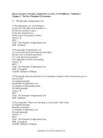
FIGURE 9.1

Aggregate Demand
The aggregate demand curve plots the total demand for real GDP as a function of the price level. The
aggregate demand curve slopes downward, indicating that the quantity of aggregate demand increases
as the price level in the economy falls.

In Figure 9.1, the aggregate demand curve is downward sloping. As the price level
falls, the total quantity demanded for goods and services increases. To understand
what the aggregate demand curve represents, we must first learn the components of
aggregate demand, why the aggregate demand curve slopes downward, and the factors
that can shift the curve.

T h e Co m po nen t s o f Ag g regat e D em and
In our study of GDP accounting, we divided GDP into four components:
consumption spending (C), investment spending (I), government purchases (G), and
net exports (NX). These four components are also the four parts of aggregate demand
because the aggregate demand curve really just describes the demand for total GDP
at different price levels. As we will see, changes in demand coming from any of these
four sources—C, I, G, or NX—will shift the aggregate demand curve.

W h y th e A g gregat e Deman d Cu rv e Slop es D ownwar d
To understand the slope of the aggregate demand curve, we need to consider the
effects of a change in the overall price level in the economy. First, let’s consider the
supply of money in the economy. We discuss the supply of money in detail in later
chapters, but for now, just think of the supply of money as being the total amount of
currency (cash plus coins) held by the public and the value of all deposits in savings
and checking accounts. As the price level or average level of prices in the economy
changes, so does the purchasing power of your money. This is an example of the
real-nominal principle.

REAL-NOMINAL PRINCIPLE
What matters to people is the real value or purchasing power of money
or income, not the face value of money or income.

189

Find more at

190

C H A P T E R 9   •   A G GREGA T E D EM A ND AND AGGREGATE SUPPLY

As the purchasing power of money changes, the aggregate demand curve is
affected in three different ways:
• The wealth effect
• The interest rate effect
• The international trade effect
Let’s take a closer look at each.

wealth effect
The increase in spending that occurs
because the real value of money increases
when the price level falls.

THE WEALTH EFFECT The increase in spending that occurs because the real value
of money increases when the price level falls is known as the wealth effect. Lower prices
lead to higher levels of wealth, and higher levels of wealth increase spending on total
goods and services. Conversely, when the price level rises, the real value of money
decreases, which reduces people’s wealth and their total demand for goods and services
in the economy. When the price level rises, consumers can’t simply substitute one good
for another that’s cheaper, because at a higher price level everything is more expensive.
THE INTEREST RATE EFFECT With a given supply of money in the economy,
a lower price level will lead to lower interest rates. With lower interest rates, both
consumers and firms will find it cheaper to borrow money to make purchases. As a

consequence, the demand for goods in the economy (consumer durables purchased by
households and investment goods purchased by firms) will increase. (We’ll explain the
effects of interest rates in more detail in later chapters.)
THE INTERNATIONAL TRADE EFFECT In an open economy, a lower price level
will mean that domestic goods (goods produced in the home country) become cheaper
relative to foreign goods, so the demand for domestic goods will increase. For
example, if the price level in the United States falls, it will make U.S. goods cheaper
relative to foreign goods. If U.S. goods become cheaper than foreign goods, exports
from the United States will increase and imports will decrease. Thus, net exports—a
component of aggregate demand—will increase.

Sh ift s in the Aggr egate Dem and C ur ve
A fall in price causes the aggregate demand curve to slope downward because of three
factors: the wealth effect, the interest rate effect, and the international trade effect.
What happens to the aggregate demand curve if a variable other than the price level
changes? An increase in aggregate demand means that total demand for all the goods
and services contained in real GDP has increased—even though the price level hasn’t
changed. In other words, increases in aggregate demand shift the curve to the right.
Conversely, factors that decrease aggregate demand shift the curve to the left—even
though the price level hasn’t changed.
Let’s look at the key factors that cause these shifts. We will discuss each factor in
detail in later chapters:
• Changes in the supply of money
• Changes in taxes
• Changes in government spending
• All other changes in demand
CHANGES IN THE SUPPLY OF MONEY An increase in the supply of money in
the economy will increase aggregate demand and shift the aggregate demand curve to
the right. We know that an increase in the supply of money will lead to higher demand
by both consumers and firms. At any given price level, a higher supply of money will

mean more consumer wealth and an increased demand for goods and services. A
decrease in the supply of money will decrease aggregate demand and shift the aggregate
demand curve to the left.


Find more at
PART 4

CHANGES IN TAXES A decrease in taxes will increase aggregate demand and shift
the aggregate demand curve to the right. Lower taxes will increase the income available
to households and increase their spending on goods and services—even though the
price level in the economy hasn’t changed. An increase in taxes will decrease aggregate
demand and shift the aggregate demand curve to the left. Higher taxes will decrease
the income available to households and decrease their spending.
CHANGES IN GOVERNMENT SPENDING At any given price level, an increase in
government spending will increase aggregate demand and shift the aggregate demand
curve to the right. For example, the government could spend more on national
defense or on interstate highways. Because the government is a source of demand
for goods and services, higher government spending naturally leads to an increase in
total demand for goods and services. Similarly, decreases in government spending will
decrease aggregate demand and shift the curve to the left.

Price level, P

ALL OTHER CHANGES IN DEMAND Any change in demand from households,
firms, or the foreign sector will also change aggregate demand. For example, if the
Chinese economy expands very rapidly and Chinese citizens buy more U.S. goods,
U.S. aggregate demand will increase. Or, if U.S. households decide they want to spend
more, consumption will increase and aggregate demand will increase. Expectations
about the future also matter. For example, if firms become optimistic about the

future and increase their investment spending, aggregate demand will also increase.
However, if firms become pessimistic, they will cut their investment spending and
aggregate demand will fall.
When we discuss factors that shift aggregate demand, we must not include any
changes in the demand for goods and services that arise from movements in the price
level. Changes in aggregate demand that accompany changes in the price level are
already included in the curve and do not shift the curve. The increase in consumer
spending that occurs when the price level falls from the wealth effect, the interest rate
effect, and the international trade effect is already in the curve and does not shift it.
Figure 9.2 and Table 9.1 summarize our discussion. Decreases in taxes, increases
in government spending, and increases in the supply of money all shift the aggregate
demand curve to the right. Increases in taxes, decreases in government spending, and
decreases in the supply of money shift it to the left. In general, any increase in demand

Increased AD
Initial AD
Decreased AD
Output, y

▲

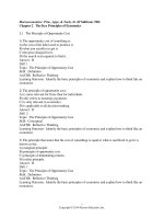
FIGURE 9.2

Shifting Aggregate Demand
Decreases in taxes, increases in government spending, and an increase in the supply of money all shift
the aggregate demand curve to the right. Higher taxes, lower government spending, and a lower supply
of money shift the curve to the left.

191

Find more at

192

C H A P T E R 9   •   A G GREGA T E D EM A ND AND AGGREGATE SUPPLY

TABLE 9.1 Factors That Shift Aggregate Demand
Factors That Increase Aggregate Demand

Factors That Decrease Aggregate Demand

Decrease in taxes
Increase in government spending
Increase in the money supply

Increase in taxes
Decrease in government spending
Decrease in the money supply

(not brought about by a change in the price level) will shift the curve to the right.
Decreases in demand shift the curve to the left.

How t h e M ultip lier M akes the Shift Bigger

multiplier

Let’s take a closer look at the shift in the aggregate demand curve and see how far
changes really make the curve shift. Suppose the government increases its spending on
goods and services by $10 billion. You might think the aggregate demand curve would

shift to the right by $10 billion, reflecting the increase in demand for these goods and
services. Initially, the shift will be precisely $10 billion. In Figure 9.3, this is depicted
by the shift (at a given price level) from a to b. But after a brief period of time, total
aggregate demand will increase by more than $10 billion. In Figure 9.3, the total shift
in the aggregate demand curve is shown by the larger movement from a to c. The ratio
of the total shift in aggregate demand to the initial shift in aggregate demand is known
as the multiplier.

Price level, P

The ratio of the total shift in aggregate
demand to the initial shift in aggregate
demand.

a

b

c
AD1

AD2

AD0

Output, y
▲

FIGURE 9.3

The Multiplier
Initially, an increase in desired spending will shift the aggregate demand curve horizontally to the right
from a to b. The total shift from a to c will be larger. The ratio of the total shift to the initial shift is known
as the multiplier.

Why does the aggregate demand curve shift more than the initial increase
in desired spending? The logic goes back to the ideas of economist John Maynard
Keynes. Here’s how it works: Keynes believed that as government spending increases
and the aggregate demand curve shifts to the right, output will subsequently increase,
too. As we saw with the circular flow in Chapter 5, increased output also means
increased income for households, as firms pay households for their labor and for
supplying other factors of production. Typically, households will wish to spend, or
consume, part of that income, which will further increase aggregate demand. It is this
additional spending by consumers, over and above what the government has already
spent, that causes the further shift in the aggregate demand curve.
The basic idea of how the multiplier works in an economy is simple. Let’s say the
government invests $10 million to renovate a federal court building. Initially, total
spending in the economy increases by this $10 million paid to a private construction
firm. The construction workers and owners are paid $10 million for their work. Suppose
the owners and workers spend $6 million of their income on new cars (although, as we


Find more at
PART 4

will see, it does not really matter what they spend it on). To meet the increased demand
for new cars, automobile producers will expand their production and earn an additional
$6 million in wages and profits. They, in turn, will spend part of this additional income—
let’s say, $3.6 million—on televisions. The workers and owners who produce televisions
will then spend part of the $3.6 million they earn, and so on.

To take a closer look at this process, we first need to look more carefully at
the behavior of consumers and how their behavior helps to determine the level of
aggregate demand. Economists have found that consumer spending depends on the
level of income in the economy. When consumers have more income, they want to
purchase more goods and services. The relationship between the level of income and
consumer spending is known as the consumption function:
C = Ca + by
where consumption spending, C, has two parts. The first part, Ca, is a constant and is
independent of income. Economists call this autonomous consumption spending.
Autonomous spending is spending that does not depend on the level of income.
For example, all consumers, regardless of their current income, will have to purchase
some food. The second part, by, represents the part of consumption that is dependent
on income. It is the product of a fraction, b, called the marginal propensity to
consume (MPC), and the level of income, or y, in the economy. The MPC (or b in
our formula) tells us how much consumption spending will increase for every dollar
that income increases. For example, if b is 0.6, then for every $1.00 that income
increases, consumption increases by $0.60.
Here is another way to think of the MPC: If a household receives some additional
income, it will increase its consumption by some additional amount. The MPC is
defined as the ratio of additional consumption to additional income, or
MPC =

consumption function
The relationship between consumption
spending and the level of income.

autonomous consumption spending
The part of consumption spending that
does not depend on income.

marginal propensity to
consume (MPC)
The fraction of additional income that
is spent.

additional consumption
additional income

For example, if the household receives an additional $100 and consumes an additional
$70, the MPC will be
+70
= 0.7
+100
You may wonder what happens to the other $30. Whatever the household does not
spend out of income, it saves. Therefore, the marginal propensity to save (MPS) is
defined as the ratio of additional savings to additional income
MPS =

additional savings
additional income

The sum of the MPC and the MPS always equals one. By definition, additional
income is either spent or saved.
Now we are in a better position to understand the multiplier. Suppose the
government increases its purchases of goods and services by $10 million. This will
initially raise aggregate demand and income by $10 million. But because income
has risen by $10 million, consumers will now wish to increase their spending by
an amount equal to the marginal propensity to consume multiplied by the
$10 million. (Remember that the MPC tells us how much consumption spending
will increase for every dollar that income increases.) If the MPC were 0.6, then

consumer spending would increase by $6 million when the government spends
$10 million. Thus, the aggregate demand curve would continue to shift to the
right by another $6 million in addition to the original $10 million, for a total of
$16 million.
But the process does not end there. As aggregate demand increases by $6 million,
income will also increase by $6 million. Consumers will then wish to increase their

marginal propensity to save (MPS)
The fraction of additional income that
is saved.

193


Find more at

194

C H A P T E R 9   •   A G GREGA T E D EM A ND AND AGGREGATE SUPPLY

spending by the MPC * $6 million or, in our example, by $3.6 million (0.6 *
$6 million). The aggregate demand curve will continue to shift to the right, now by
another $3.6 million. Adding $3.6 million to $16 million gives us a new aggregate
demand total of $19.6 million. As you can see, this process will continue, as consumers
now have an additional $3.6 million in income, part of which they will spend again.
Where will it end?
Table 9.2 shows how the multiplier works in detail. In the first round, there is
an initial increase in government spending of $10 million. This additional demand
leads to an initial increase in GDP and income of $10 million. Assuming that the
MPC is 0.6, the $10 million of additional income will increase consumer spending by

$6 million. The second round begins with this $6 million increase in consumer spending.
Because of this increase in demand, GDP and income increase by $6 million. At the end
of the second round, consumers will have an additional $6 million; with an MPC of 0.6,
consumer spending will therefore increase by 0.6 * $6 million, or $3.6 million. The
process continues in the third round with an increase in consumer spending of
$2.16 million. It continues, in diminishing amounts, through subsequent rounds. If we
add up the spending in all the (infinite) rounds, we will find that the initial $10 million of
spending leads to a $25 million increase in GDP and income. That’s 2.5 times what the
government initially spent. So in this case, the multiplier is 2.5.

TABLE 9.2 THE MULTIPLIER IN ACTION
The initial $10 million increase in aggregate demand will, through all the rounds
of spending, eventually lead to a $25 million increase.
Round of Spending

Increase in Aggregate
Demand (millions)

Increase in GDP and
Income (millions)

Increase in
Consumption (millions)

1
2
3
4
.
Total

$10.00
6.00
3.60
2.16
.
$25.00

$10.00
6.00
3.60
2.16
.
$25.00

$6.00
3.60
2.16
1.30
.
$15.00

Instead of calculating spending round by round, we can use a simple formula to
figure out what the multiplier is:
multiplier =

1
11 - MPC 2

Thus, in the preceding example, when the MPC is 0.6, the multiplier would be

1
= 2.5
11 - 0.62
Now you should clearly understand why the total shift in the aggregate demand
curve from a to c in Figure 9.3 is greater than the initial shift in the curve from
a to b. This is the multiplier in action. The multiplier is important because it means
that relatively small changes in spending could lead to relatively large changes in
output. For example, if firms cut back on their investment spending, the effects on
output would be “multiplied,” and this decrease in spending could have a large,
adverse impact on the economy.
In practice, once we take into account other realistic factors such as taxes and
indirect effects through financial markets, the multipliers are smaller than our
previous examples, typically near 1.5 for the U.S economy. This means that a
$10 million increase in one component of spending will shift the U.S. aggregate
demand curve by approximately $15 million. Some economists believe the multiplier


Find more at
PART 4

is even closer to one. Knowing the value of the multiplier is important for two reasons. First, it tells us how much shocks to aggregate demand are “amplified.” Second,
to design effective economic policies to shift the aggregate demand curve, we need to
know the value of the multiplier to measure the proper “dose” for policy. In the next
chapter, we present a more detailed model of aggregate demand and see how policymakers use the real-world multipliers.

application 2
TWO APPROACHES TO DETERMINING THE CAUSES OF
RECESSIONS
APPLYING THE CONCEPTS #2: How can we determine what factors cause
recessions?

Economists have used the basic framework of aggregate demand and supply analysis
to explain recessions. Recessions can occur either when there is a sharp decrease in
aggregate demand—a leftward shift in the aggregate demand curve—or a decrease
in aggregate supply—an upward shift in the short-run aggregate supply curve. But
this just puts the question back one level: During particular historical episodes, what
actually shifted the curves?
Figuring out what caused a recession in any particular episode is very challenging.
Here is one complication. Policymakers typically respond to shocks that hit the
economy. So, for example, when worldwide oil prices rose in 1973 causing U.S. prices
to increase, policymakers also reduced aggregate demand to prevent further price
increases. Was the recession that resulted due to (1) the increase in oil prices that
shifted the short-run aggregate supply curve or (2) the decrease in aggregate demand
engineered by policymakers? It is very difficult to know.
One approach is to use economic models to address this question. Economists James
Fackler and Douglas McMillin built a small model of the economy to address this issue.
To distinguish between demand and supply shocks, they used an idea that we discuss in
this chapter. Shocks to aggregate demand only affect prices in the long run but do not
affect output. On the other hand, shocks to aggregate supply can affect potential output
in the long run. Using this approach, they find that a mixture of demand and supply
shocks were responsible for fluctuations in output in the United States.
Using more traditional historical methods, economic historian Peter Temin
looked back at all recessionary episodes from 1893 to 1990 in the United States to try
to determine their ultimate causes. According to his analysis, recessions were caused by
many different factors. Sometimes, as in 1929, they were caused by shifts in aggregate
demand from the private sector, as consumers cut back their spending. Other times,
as in 1981, the government cut back on aggregate demand to reduce inflation. Supply
shocks were the cause of the recessions in 1973 and 1979.
Based on both economic models and traditional economic history, it does
appear that both supply and demand shocks have been important in understanding
recessions. Related to Exercises 3.6 and 3.9.

SOURCE: Based on Peter Temin, “The Causes of American Business Cycles: An Essay in Economic Historiography,” in
Federal Reserve Bank of Boston Conference Series 42, Beyond Shocks: What Causes Business Cycles, />economic/conf/conf42 (accessed April 12, 2010), and James Fackler and Douglas McMillin, “Historical Decomposition
of Aggregate Demand and Supply Shocks in a Small Macro Model,” Southern Economic Journal 64, no. 3 (1998): 648–684.

195


Find more at

196

C H A P T E R 9   •   A G GREGA T E D EM A ND AND AGGREGATE SUPPLY

9.3
aggregate supply curve (AS)
A curve that shows the relationship
between the level of prices and the
quantity of output supplied.

Understanding Aggregate Supply

Now we turn to the supply side of our model. The aggregate supply curve (AS)
shows the relationship between the level of prices and the total quantity of final goods
and output that firms are willing and able to supply. The aggregate supply curve will
complete our macroeconomic picture, uniting the economy’s demand for real output
with firms’ willingness to supply output. To determine both the price level and real
GDP, we need to combine both aggregate demand and aggregate supply. One slight
complication is that because prices are “sticky” in the short run, we need to develop
two different aggregate supply curves, one corresponding to the long run and one to
the short run.

T h e L o n g -Run Aggr egate Sup p ly C ur v e
long-run aggregate supply curve
A vertical aggregate supply curve that
reflects the idea that in the long run,
output is determined solely by the factors
of production and technology.

▶

First we’ll consider the aggregate supply curve for the long run, that is, when the
economy is at full employment. This curve is also called the long-run aggregate
supply curve. In previous chapters, we saw that the level of full-employment output,
yp (the “p” stands for potential), depends solely on the supply of factors—capital,
labor—and the state of technology. These are the fundamental factors that determine
output in the long run, that is, when the economy operates at full employment.
In the long run, the economy operates at full employment and changes in the price
level do not affect employment. To illustrate why this is so, imagine that the price level
in the economy increases by 50 percent. That means firms’ prices, on average, will also
increase by 50 percent. However, so will their input costs. Their profits will be the same
and, consequently, so will their output. Because the level of full-employment output
does not depend on the price level, we can plot the long-run aggregate supply curve as a
vertical line (unaffected by the price level), as shown in Figure 9.4.

FIGURE 9.4

Long-run AS

Long-Run Aggregate Supply

Price level, P

In the long run, the level of output, yp, is
independent of the price level.

yp
Output

DETERMINING OUTPUT AND THE PRICE LEVEL We combine the aggregate
demand curve and the long-run aggregate supply curve in Figure 9.5. Together, the
curves show us the price level and output in the long run when the economy returns to
full employment. Combining the two curves will enable us to understand how changes
in aggregate demand affect prices in the long run.
The intersection of an aggregate demand curve and an aggregate supply curve
determines the price level and equilibrium level of output. At that intersection point,
the total amount of output demanded will just equal the total amount supplied by
producers—the economy will be in macroeconomic equilibrium. The exact position


Find more at
PART 4

Price level, P

Long-run AS

Increased AD
Initial AD
yp
Output

▲

FIGURE 9.5

Aggregate Demand and the Long-Run Aggregate Supply
Output and prices are determined at the intersection of AD and AS. An increase in aggregate demand
leads to a higher price level.

of the aggregate demand curve will depend on the level of taxes, government
spending, and the supply of money, although it will always slope downward. The level
of full-employment output determines the long-run aggregate supply curve.
An increase in aggregate demand (perhaps brought about by a tax cut or an increase
in the supply of money) will shift the aggregate demand curve to the right, as shown in
Figure 9.5. In the long run, the increase in aggregate demand will raise prices but leave
the level of output unchanged. In general, shifts in the aggregate demand curve in the
long run do not change the level of output in the economy, but only change the level
of prices. Here is an important example to illustrate this idea: If the money supply is
increased by 5 percent a year, the aggregate demand curve will also shift by 5 percent
a year. In the long run, this means that prices will increase by 5 percent a year—that is,
there will be 5 percent inflation. An important lesson: In the long run, increases in the
supply of money do not increase real GDP—they only lead to inflation.
This is the key point about the long run: In the long run, output is determined
solely by the supply of human and physical capital and the supply of labor, not the price
level. As our model of the aggregate demand curve with the long-run aggregate supply
curve indicates, changes in demand will affect only prices, not the level of output.

T h e S h o r t- Ru n Agg regat e Su pply C ur ve
In the short run, prices are sticky (slow to adjust) and output is determined primarily
by demand. This is what Keynes thought happened during the Great Depression. We
can use the aggregate demand curve combined with a short-run aggregate supply

curve to illustrate this idea. Figure 9.6 shows a relatively flat short-run aggregate supply curve (AS). The short-run aggregate supply curve shows the short-run relationship
between the price level and the willingness of firms to supply output to the economy.
Let’s look first at its slope and then the factors that shift the curve.
The short-run aggregate supply curve has a relatively flat slope because we
assume that in the short run firms supply all the output demanded, with small changes
in prices. We’ve said that with formal and informal contracts firms will supply all the
output demanded with only relatively small changes in prices. The short-run aggregate
supply curve has a small upward slope. As firms supply more output, they may have
to increase prices somewhat if, for example, they have to pay higher wages to obtain
more overtime from workers or pay a premium to obtain some raw materials. Our
description of the short-run aggregate supply curve is consistent with evidence about

short-run aggregate supply curve
A relatively flat aggregate supply curve
that represents the idea that prices do
not change very much in the short run
and that firms adjust production to meet
demand.

197


Find more at

Short-run AS
Price level, P

198

C H A P T E R 9   •   A G GREGA T E D EM A ND AND AGGREGATE SUPPLY

a1
a0
Increased AD

Initial AD
y0

y1
Output, y

▲

FIGURE 9.6

Aggregate Demand and Short-Run Aggregate Supply
With a short-run aggregate supply curve, shifts in aggregate demand lead to large changes in output but
small changes in price.

the behavior of prices in the economy. Most studies find that changes in demand
have relatively little effect on prices within a few quarters. Thus, we can think of the
aggregate supply curve as relatively flat over a limited time.
The position of the short-run supply curve will be determined by the costs of
production that firms face. Higher costs will shift up the short-run aggregate supply curve,
while lower costs will shift it down. Higher costs will shift up the curve because, faced with
higher costs, firms will need to raise their prices to continue to make a profit. What factors
determine the costs firms must incur to produce output? The key factors are
• input prices (wages and materials),
• the state of technology, and
• taxes, subsidies, or economic regulations.

Increases in input prices (for example, from higher wages or oil prices) will increase
firms’ costs. This will shift up the short-run aggregate supply curve. Improvement in
technology will shift the curve down. Higher taxes or more onerous regulations raise
costs and shift the curve up, while subsidies to production shift the curve down. As we
shall see later in this chapter, when the economy is not at full employment, wages and
other costs will change. These changes in costs will shift the entire short-run supply
curve upward or downward as costs rise or fall.
The intersection of the AD and AS curves at point a0 determines the price level and
the level of output. Because the aggregate supply curve is flat, aggregate demand primarily
determines the level of output. In Figure 9.6, as aggregate demand increases, the new
equilibrium will be at a slightly higher price, and output will increase from y0 to y1.
If the aggregate demand curve moved to the left, output would decrease. If the
leftward shift in aggregate demand were sufficiently large, it could push the economy
into a recession. Sudden decreases in aggregate demand have been important causes of
recessions in the United States. However, the precise factors that shift the aggregate
demand curve in each recession will typically differ.
Note that the level of output where the aggregate demand curve intersects the
short-run aggregate supply curve need not correspond to full-employment output.
Firms will produce whatever is demanded. If demand is very high and the economy is
“overheated,” output may exceed full-employment output. If demand is very low and the
economy is in a slump, output will fall short of full-employment output. Because prices
do not adjust fully over short periods of time, the economy need not always remain at


Find more at
PART 4

application 3
OIL SUPPLY DISRUPTIONS, SPECULATION AND SUPPLY
SHOCKS

APPLYING THE CONCEPTS #3: Are oil price increases caused by true shocks
to supply?
Economists have long believed that disruptions to oil supplies were the cause of supply
shocks for the U.S economy. If this were the case, supply disruptions would be true
external “shocks” to the economy. But not all changes in oil prices are necessarily
caused by supply disruptions. Oil price increases may be caused by increases in world
demand or due to the activities of speculators in the oil market.
How important are actual supply disruptions to oil market for the U.S. economy?
Economist Lutz Kilian carefully examined this issue by constructing measures of
supply disruptions in oil producing countries, based on a detailed examination of prior
trends in demand and specifications in oil contracts. While Kilian did find evidence of
some supply disruptions, these only explained a small fraction of the variability of oil
prices. In his view, other factors dominated the price movements for oil, even during
the time periods that are conventionally associated with supply disruptions.
Speculation in oil markets may be one such factor. Speculators can be countries,
firms, or individuals. If speculators believe prices are going to rise in the future, they
will buy oil now or, if they own it, sell less into the market. Either action increases the
current price of oil. Note that if speculators are on average correct in their assessments,
they will smooth out the price of oil over time—raising it now and lowering it later.
This can actually benefit the economy. While politicians often complain about
speculators, in many cases they may be helping the economy. Of course, speculators
can be wrong and make fluctuations in prices worse, but in this case at least some of
them will lose money. Related to Exercises 3.4 and 3.7.
SOURCE: In part based on Lutz Kilian, “Exogenous Oil Supply Shocks: How Big Are They and How Much Do They
Matter for the U.S. Economy?” Review of Economics and Statistics, May 2008, Vol. 90, No. 2, pp. 216–240.

full employment or potential output. With sticky prices, changes in demand in the short
run will lead to economic fluctuations and over- and underemployment. Only in the
long run, when prices fully adjust, will the economy operate at full employment.

Su ppl y S h o cks
Up to this point, we have been exploring how changes in aggregate demand affect output
and prices in the short run and in the long run. However, even in the short run, it is possible
for external disturbances to hit the economy and cause the short-run aggregate supply
curve to move. Supply shocks are external events that shift the aggregate supply curve.
The most notable supply shocks for the world economy occurred in 1973 and
again in 1979 when oil prices increased sharply. Oil is a vital input for many companies
because it is used to both manufacture and transport their products to warehouses and
stores around the country. The higher oil prices raised firms’ costs and reduced their
profits. To maintain their profit levels, firms raised their product prices. As we have
seen, increases in firms’ costs will shift up the short-run aggregate supply curve—
increases in oil prices are a good example.
Figure 9.7 illustrates a supply shock that raises prices. The short-run aggregate
supply curve shifts up with the supply shock because, as their costs rise, firms will supply
their output only at a higher price. The AS curve shifts up, raising the price level and
lowering the level of output from y0 to y1. Adverse supply shocks can therefore cause a
recession (a fall in real output) with increasing prices. This phenomenon is known as

supply shocks
External events that shift the aggregate
supply curve.

199


Find more at

200

C H A P T E R 9   •   A G GREGA T E D EM A ND AND AGGREGATE SUPPLY

Price level, P

AS (after the shock)

AS (before the shock)

AD

y1

y0
Output, y

▲

FIGURE 9.7

Supply Shock
An adverse supply shock, such as an increase in the price of oil, will cause the AS curve to shift upward.
The result will be higher prices and a lower level of output.

stagflation
A decrease in real output with increasing
prices.

stagflation, and it is precisely what happened in 1973 and 1979. The U.S. economy
suffered on two grounds: rising prices and falling output. Favorable supply shocks,
such as falling prices, are also possible, and changes in oil prices can affect aggregate
demand.

9.4

From the Short Run to the Long Run

Up to this point, we have examined how aggregate demand and aggregate supply
determine output and prices both in the short run and in the long run. You may be
wondering how long it takes before the short run becomes the long run. Here is a
preview of how the short run and the long run are connected.
In Figure 9.8, we show the aggregate demand curve intersecting the short-run
aggregate supply curve at a0 at an output level y0. We also depict the long-run aggregate
supply curve in this figure. The level of output in the economy, y0, exceeds the level of
potential output, yp. In other words, this is a boom economy: Output exceeds potential.
▶

FIGURE 9.8

Long-run AS

The Economy in the Short Run
In the short run, the economy produces
at y0, which exceeds potential output yp.

Price level, P

Short-run AS

a0

AD

yp

y0
Output, y


Find more at
PART 4

What happens during a boom? Because the economy is producing at a level
beyond its long-run potential, the level of unemployment will be very low. This will
make it difficult for firms to recruit and retain workers. Firms will also find it more
difficult to purchase needed raw materials and other inputs for production. As firms
compete for labor and raw materials, the tendency will be for both wages and prices
to increase over time.
Increasing wages and prices will shift the short-run aggregate supply curve
upward as the costs of inputs rise in the economy. Figure 9.9 shows how the short-run
aggregate supply curve shifts upward over time. As long as the economy is producing
at a level of output that exceeds potential output, there will be continuing competition
for labor and raw materials that will lead to continuing increases in wages and prices.
In the long run, the short-run aggregate supply curve will keep rising until it intersects
the aggregate demand curve at a1. At this point, the economy reaches the long-run
equilibrium—precisely the point where the aggregate demand curve intersects the
long-run aggregate supply curve.
Long-run AS
AS3
AS2

a1

Price level, P

AS1
AS0

a0
AD

yp

y0
Output, y

▲

FIGURE 9.9

Adjusting to the Long Run
With output exceeding potential, the short-run AS curve shifts upward over time. The economy adjusts
to the long-run equilibrium at a1.

When the economy is producing below full employment or potential output, the
process works in reverse. Unemployment will exceed the natural rate, and there will be
excess unemployment. Firms will find it easy to hire and retain workers, and they will
offer workers less wages. As firms cut wages, the average wage level in the economy
falls. Because wages are the largest component of costs and costs are decreasing, the
short-run aggregate supply curve shifts down, causing prices to fall as well.
The lesson here is that adjustments in wages and prices take the economy from the
short-run equilibrium to the long-run equilibrium. In later chapters, we will explain in
detail how this adjustment occurs, and we will show how changes in wages and prices

can steer the economy back to full employment in the long run.
The aggregate demand and aggregate supply model in this chapter provides an
overview of how demand affects output and prices in both the short run and the long
run. We will expand our discussion of aggregate demand to see in detail how such
realistic and important factors as spending by consumers and firms, government
policies on taxation and spending, and foreign trade affect the demand for goods and
services. We will also study the critical role that the financial system and monetary
policy play in determining demand. Finally, we will study in more depth how the
aggregate supply curve shifts over time, enabling the economy to recover both from
recessions and the inflationary pressures generated by economic booms.

201


Find more at

SUMMARY
In this chapter we discussed
how sticky prices—or lack
of full-wage and price flexibility—cause output to be
determined by demand in the
short run. We developed a
model of aggregate demand
and supply to help us analyze
what is happening or has happened in the economy. Here are the
main points in this chapter:
1 Because prices are sticky in the short run, economists think of
GDP as being determined primarily by demand factors in the
short run.
2 The aggregate demand curve depicts the relationship between

the price level and total demand for real output in the economy.
The aggregate demand curve is downward sloping because of
the wealth effect, the interest rate effect, and the international
trade effect.
3 Decreases in taxes, increases in government spending, and
increases in the supply of money all increase aggregate demand
and shift the aggregate demand curve to the right. Increases
in taxes, decreases in government spending, and decreases in

the supply of money all decrease aggregate demand and shift
the  aggregate demand curve to the left. In general, anything
(other than price movements) that increases the demand for total
goods and services will increase aggregate demand.
4 The total shift in the aggregate demand curve is greater than the
initial shift. The ratio of the total shift in aggregate demand to the
initial shift in aggregate demand is known as the multiplier.
5 The aggregate supply curve depicts the relationship between
the price level and the level of output that firms supply in the
economy. Output and prices are determined at the intersection
of the aggregate demand and aggregate supply curves.
6 The long-run aggregate supply curve is vertical because, in the
long run, output is determined by the supply of factors of production. The short-run aggregate supply curve is fairly flat because,
in the short run, prices are largely fixed, and output is determined
by demand. The costs of production determine the position of
the short-run aggregate supply curve.
7 Supply shocks can shift the short-run aggregate supply curve.
8 As costs change, the short-run aggregate supply curve shifts
in the long run, restoring the economy to the full-employment
equilibrium.

KEY TERMS
aggregate demand curve (AD), p. 188

marginal propensity to consume
(MPC), p. 193

short-run aggregate supply curve,

aggregate supply curve (AS), p. 196
autonomous consumption spending,

marginal propensity to save (MPS),

stagflation, p. 200

p. 193

p. 193

p. 197

supply shocks, p. 199

consumption function, p. 193

multiplier, p. 192

long-run aggregate supply curve,

short run in macroeconomics, p. 187

wealth effect, p. 190

p. 196

EXERCISES

9.1
1.1

1.2
1.3

202

All problems are assignable in MyEconLab; exercises that update with real-time data are marked with

Sticky Prices and Their Macroeconomic
Consequences

Arthur Okun distinguished between auction prices,
which changed rapidly, and
prices,
which are slow to change.
For most firms, the biggest cost of doing business is
.
The price system always coordinates economic
activity, even when prices are slow to adjust to changes
in demand and supply.
(True/False)

1.4

1.5

.

Determine whether the wages of each of the following
adjust slowly or quickly to changes in demand and
supply.
a. Union workers
b. Internationally known movie stars or rock stars
c. University professors
d. Athletes
The Internet and Price Flexibility. The Internet
enables consumers to search for the lowest prices of
various goods, such as books, music CDs, and airline
tickets. Prices for these goods are likely to become
more flexible as consumers shop around quickly


Find more at

1.6

1.7

1.8

and easily on the Internet. What types of goods and

services do you think may not become more flexible
because of the Internet? Give an example of a good
or service for which you have searched the Internet
for price information and one for which you have not.
(Related to Application 1 on page 188.)
Airlines and Stable Fuel Prices. Southwest Airlines
made it a company policy to engage in complex
financial transactions to keep the cost of fuel constant.
Why would the airline want to have stable fuel prices?
Supermarket Prices. In a supermarket, prices for
tomatoes change quickly, but prices for mops tend to
not change as rapidly. Can you offer an explanation
why? (Related to Application 1 on page 188.)
Retail Price Stickiness in Catalogs. During periods
of high inflation, retail prices in catalogs changed
more frequently. Explain why this occurred. (Related
to Application 1 on page 188.)

9.2
2.1

2.2

2.3

2.4
2.5

2.6

2.7

2.8

2.9

9.3
3.1
3.2
3.3

Understanding Aggregate Demand

Which of the following is not a component of
aggregate demand?
a. Consumption
b. Investment
c. Government expenditures
d. The supply of money
e. Net exports
In the Great Depression, prices in the United States
fell by 33 percent. Ceteris paribus, this led to an increase
in aggregate demand through three channels: the
effect, the interest rate effect, and
the international trade effect.
President Barack Obama lowered taxes in 2009. He
also increased government spending. Ceteris paribus,
these actions shifted the aggregate demand curve to
the
.

If the MPC is 0.8, the simple multiplier will be
.
Because of other economic factors, such as taxes, the
multiplier in the United States is
(larger/
smaller) than 2.5.
Opening Export Markets. Suppose a foreign
country, which originally prevented the United States
from exporting to it, opens its market and U.S. firms
start to make a considerable volume of sales. What
happens to the aggregate demand curve?
Calculating the MPS and MPC. In one year, a
consumer’s income increases by $200 and her savings
increases by $40. What is her marginal propensity to
save. What is her marginal propensity to consume?

Saving Behavior and Multipliers in Two Countries.
Consumers in Country A have an MPS of 0.5 while
consumers in Country B have an MPS of 0.4. Which
country has the higher value for the multiplier?
State and Local Governments during Recessions.
During recessions, state governments often will have
to raise taxes and cut spending in order to keep their
own budgets balanced. If a large number of states do
this, what will happen to the aggregate demand curve
at the national level?

3.4

3.5

3.6

3.7

3.8

Understanding Aggregate Supply

The long-run aggregate supply curve is
(vertical/horizontal).
A decrease in material costs will shift the short-run
aggregate supply
.
Using the long-run aggregate supply curve, a decrease
in aggregate demand will
prices and
output.
A negative supply shock, such as higher oil prices, will
output and
prices in the
short run. (Related to Application 3 on page 199.)
Higher Gas Prices, Frugal Consumers, and
Economic Fluctuations. Suppose gasoline prices
increased sharply and consumers became fearful of
owning too many expensive cars. As a consequence,
they cut back on their purchases of new cars and
decided to increase their savings. How would this
behavior shift the aggregate demand curve? Using the
short-run aggregate supply curve, what will happen to

prices and output in the short run?
What Caused This Recession? Suppose the
economy goes into a recession. The political party
in power blames it on an increase in the price of
world oil and food. Opposing politicians blame a tax
increase that the party in power had enacted. On
the basis of aggregate demand and aggregate supply
analysis, what evidence should you look at to try to
determine what, or who, caused the recession? (Hint:
look at the behavior of both prices and output in each
case.) (Related to Application 2 on page 195.)
The Role of Expectations and Supply Shocks.
Suppose an oil producing country believed that
political instability was likely in the future in other
parts of the world and prices would rise in the next
year. Do you think they would sell more or less
today? What will happen to today’s price? Will this
affect either aggregate demand or supply? (Related to
Application 3 on page 199.)
China Comes Roaring Back. In the 2008 recession,
China was one of the first economies to recover and
its GDP growth quickly returned to its pre-recession
203


Find more at

3.9

levels. How did China’s actions affect aggregate

demand in the rest of the world?
Long-Run Effects of a Shock to Demand. Suppose
consumption spending rose quickly and then fell back
to its normal level. What do you think would be the
long-run effect on real GDP of this temporary shock?
(Related to Application 2 on page 195.)

4.4

4.5

9.4
4.1

4.2

4.3

204

From the Short Run to the Long Run

Suppose the supply of money increases, causing
output to exceed full employment. Prices will
and real GDP will
in the
short run, and prices will
and real GDP
will
in the long run.

Consider a decrease in the supply of money that causes
output to fall short of full employment. Prices will
and real GDP will
in the
short run, and prices will
and real GDP
will
in the long run.
In a recession, real GDP is
potential GDP.
This implies that unemployment is
the
. This results in
natural rate, driving wages
a(n) shift of the short-run aggregate supply curve.

4.6

4.7

A negative supply shock temporarily lowers output
below full employment and raises prices. After the
negative supply shock, real GDP is
potential GDP. This implies that unemployment is
the natural rate, driving up wages. This
results in a(n)
shift of the short-run
aggregate supply curve.
The Internet Crashes. Suppose that computer
hackers managed to crash the Internet in the United

States for a week and no one had computer access.
Explain why this might be considered a negative
supply shock.
Shifts in Aggregate Demand and Cost-Push
Inflation. When wages rise and the short-run
aggregate supply curve shifts up, the result is
“cost-push” inflation. If the economy was initially at
full-employment and the aggregate demand curve was
shifted to the right, explain how “cost-push” inflation
would result as the economy adjusts back to full
employment.
Exports and Real GDP. Are increases in exports
associated with increases in real GDP? A good place
to start to find out is the Web site of the Federal
Reserve Bank of St. Louis (ouisfed.
org/fred2).


Find more at

CHAPTER

10

Fiscal Policy
Economists generally believe that permanent
tax cuts will stimulate the economy and lead
to higher output, but disagree about why this
happens.

Some advocates for tax cuts stress how they lead to increases in
spending and aggregate demand. Others suggest that the main
effect comes from changes in incentives and aggregate supply.
Can we tell which view is correct by looking back at U.S. fiscal
history? The tax cuts proposed by President John F. Kennedy and
enacted after his death are typically viewed as triumphs of the aggregate demand view. Kennedy’s economic advisers believed that tax
cuts worked through changing aggregate demand. On the other
hand, President Ronald Reagan is famously known for his “supply side” economics. His economic advisers placed
great emphasis on how cutting tax rates would create a better economic climate through improved economic
incentives.
But the economic policy world is not that simple. Kennedy’s tax cuts included incentives to increase aggregate
supply, including cutting the top income tax rate and providing specific tax incentives for business investments.
While Reagan’s tax cuts lowered tax rates for everyone, they also directly increased household incomes, which
led to more spending. A careful look at actual policies suggests that tax cuts are always a mixture of demand and
supply elements.
Today, proponents of permanent tax cuts typically cite both the Kennedy and Reagan administrations
as evidence that tax cuts work, regardless of their own view. By associating themselves with past successes,
proponents of tax cuts hope to benefit from the favorable glow of history.

LEARNING OBJECTIVES
•

Explain how fiscal policy works using
aggregate demand and aggregate supply.

•

Identify the main elements of spending and
revenue for the U.S. federal government.

•

Discuss the key episodes of active fiscal
policy in the U.S. since World War II.

MyEconLab

MyEconLab helps you master each objective and
study more efficiently.

205


Find more at

206

C H A P T E R 1 0   •   F I SCAL POL ICY

fiscal policy
Changes in government taxes and
spending that affect the level of GDP.

w

hen the U.S. economy began to slow in late 2007 and early 2008, it was
not long before policymakers and politicians from both major parties
were calling for government action to combat the downturn. Common
prescriptions included increasing government spending or reducing taxes, although
specific recommendations differed sharply among those making them. Even after the

recession ended and the slow recovery began, there were still some calls for additional
action to stimulate the economy.
In this chapter, we study how governments can use fiscal policy—changes in taxes
and spending that affect the level of GDP—to stabilize the economy. We explore the
logic of fiscal policy and explain why changes in government spending and taxation
can, in principle, stabilize the economy. However, stabilizing the economy is much
easier in theory than in actual practice, as we will see.
The chapter also provides an overview of spending and taxation by the federal
government. These are essentially the tools the government uses to implement its fiscal
policies. We will examine the federal deficit and begin to explore the controversies
surrounding deficit spending.
One of the best ways to really understand fiscal policy is to see it in action. In
the last part of the chapter, we trace the history of U.S. fiscal policy from the Great
Depression in the 1930s to the present. As you will see, the public’s attitude toward
government fiscal policy has not been constant but has instead changed over time.

10.1 The Role of Fiscal Policy
In the last chapter, we discussed how output and prices are determined where the
aggregate demand curve intersects the short-run aggregate supply curve. In this
section, we will explore how the government can shift the aggregate demand curve.

F is cal Policy and Aggr egate D em and
As we discussed in the last chapter, government spending and taxes can affect the
level of aggregate demand. Increases in government spending or decreases in taxes
will increase aggregate demand and shift the aggregate demand curve to the right.
Decreases in government spending or increases in taxes will decrease aggregate
demand and shift the aggregate demand curve to the left.
Why do changes in government spending or taxes shift the aggregate demand
curve? Recall from our discussion in the last chapter that aggregate demand consists
of four components: consumption spending, investment spending, government

purchases, and net exports. These four components are the four parts of aggregate
demand. Thus, increases in government purchases directly increase aggregate demand
because they are a component of aggregate demand. Decreases in government
purchases directly decrease aggregate demand.
Changes in taxes affect aggregate demand indirectly. For example, if the
government lowers taxes consumers pay, consumers will have more income at
their disposal and will increase their consumption spending. Because consumption
spending is a component of aggregate demand, aggregate demand will increase as
well. Increases in taxes will have the opposite effect. Consumers will have less income
at their disposal and will decrease their consumption spending. As a result, aggregate
demand will decrease. Changes in taxes can also affect businesses and lead to changes
in investment spending. Suppose, for example, that the government cuts taxes in such
a way as to provide incentives for new investment spending by businesses. Because
investment spending is a component of aggregate demand, the increase in investment
spending will increase aggregate demand.
In Panel A of Figure 10.1 we show a simple example of fiscal policy in action.
The economy is initially operating at a level of GDP, y0, where the aggregate demand
curve AD0 intersects the short-run aggregate supply curve AS. This level of output


Find more at

AD1

AD1

AD0

Short-run AS

y0

Output, y
(A)
▲

Short-run AS

yp

yp

AD0

Price level, P

Price level, P

PART 4

y0
Output, y
(B)

FIGURE 10.1

Fiscal Policy in Action
Panel A shows that an increase in government spending shifts the aggregate demand curve from AD0 to AD1,
restoring the economy to full employment. This is an example of expansionary policy. Panel B shows that an
increase in taxes shifts the aggregate demand curve to the left, from AD0 to AD1, restoring the economy to full

employment. This is an example of contractionary policy.

is below the level of full employment or potential output, yp. To increase the level of
output, the government can increase government spending—say, on military goods—
which will shift the aggregate demand curve to the right, to AD1. Now the new
aggregate demand curve intersects the aggregate supply curve at the full-employment
level of output. Alternatively, instead of increasing its spending, the government
could reduce taxes on consumers and businesses. This would also shift the aggregate
demand curve to the right. Government policies that increase aggregate demand are
called expansionary policies. Increasing government spending and cutting taxes are
examples of expansionary policies.
The government can also use fiscal policy to decrease GDP if the economy is
operating at too high a level of output, which would lead to an overheating economy
and rising prices. In Panel B of Figure 10.1, the economy is initially operating at a
level of output, y0, that exceeds full-employment output, yp. An increase in taxes can
shift the aggregate demand curve from AD0 to AD1. This shift will bring the economy
back to full employment.
Alternatively, the government could cut its spending to move the aggregate
demand curve to the left. Government policies that decrease aggregate demand are
called contractionary policies. Decreasing government spending and increasing
taxes are examples of contractionary policies.
Both examples illustrate how policymakers use fiscal policy to stabilize the
economy. In these two simple examples, fiscal policy seems very straightforward. But
as we will soon see, in practice it is more difficult to implement effective policy.

T h e F i sc a l Mu lt iplier
Let’s recall the multiplier we developed in the last chapter. The basic idea is that the final
shift in the aggregate demand curve will be larger than the initial increase. For example,
if government purchases increased by $10 billion, that would initially shift the aggregate demand curve to the right by $10 billion. However, the total shift in the aggregate
demand curve will be larger, say, $15 billion. Conversely, a decrease in purchases by

$10 billion may cause a total shift of the aggregate demand curve to the left by $15 billion.

expansionary policies
Government policy actions that lead to
increases in aggregate demand.

contractionary policies
Government policy actions that lead to
decreases in aggregate demand.

207


Find more at

208

C H A P T E R 1 0   •   F I SCAL POL ICY

This multiplier effect occurs because an initial change in output will affect the
income of households and thus change consumer spending. For example, an increase
in government spending of $10 billion will initially raise household incomes by
$10 billion and lead to increases in consumer spending. As we discussed in the last
chapter, the precise amount of the increase will depend on the marginal propensity
to consume and other factors. In turn, the increase in consumer spending will raise
output and income further, leading to further increases in consumer spending. The
multiplier takes all these effects into account.
As the government develops policies to stabilize the economy, it needs to take
the multiplier into account. The total shift in aggregate demand will be larger than
the initial shift. As we will see later in this chapter, U.S. policymakers have taken the

multiplier into account as they have developed policies for the economy.

T h e L imits to Stab iliz ation Policy

stabilization policies
Policy actions taken to move the economy
closer to full employment or potential
output.

inside lags
The time it takes to formulate a policy.

outside lags
The time it takes for the policy to
actually work.

We’ve seen that the government can use fiscal policy—changes in the level of taxes or
government spending—to alter the level of GDP. If the current level of GDP is below
full employment or potential output, the government can use expansionary policies, such
as tax cuts and increased spending, to raise the level of GDP and reduce unemployment.
Both expansionary and contractionary policies are examples of stabilization
policies, actions to move the economy closer to full employment or potential output.
It is very difficult to implement stabilization policies for two big reasons. First,
there are lags, or delays, in stabilization policy. Lags arise because decision makers are
often slow to recognize and respond to changes in the economy, and fiscal policies and
other stabilization policies take time to operate. Second, economists simply do not know
enough about all aspects of the economy to be completely accurate in all their forecasts.
Although economists have made great progress in understanding the economy, the
difficulties of forecasting the precise behavior of human beings, who can change their
minds or sometimes act irrationally, place limits on our forecasting ability.

LAGS Poorly timed policies can magnify economic fluctuations. Suppose that
(1) GDP is currently below full employment but will return to full employment on its
own within one year, and that (2) stabilization policies take a full year to become effective.
If policymakers tried to expand the economy today, their actions would not take effect
until a year from now. One year from now, the economy would normally be back at full
employment by itself. But if stabilization policies were enacted, one year from now the
economy would be stimulated unnecessarily, and output would exceed full employment.
Figure 10.2 illustrates the problem caused by lags. Panel A shows an example of
successful stabilization policy. The solid line represents the behavior of GDP in the
absence of policies. Successful stabilization policies can dampen, that is, reduce in
magnitude, economic fluctuations, lowering output when it exceeds full employment
and raising output when it falls below full employment. This would be easy to
accomplish if there were no lags in policy. The dashed curve shows how successful
policies can reduce economic fluctuations.
Panel B shows the consequences of ill-timed policies. Again, assume that policies
take a year before they are effective. At the start of year 0, the economy is below
potential. If policymakers engaged in expansionary policies at the start of year 1, the
change would not take effect until the end of year 1. This would raise output even
higher above full employment. Ill-timed stabilization policies can magnify economic
fluctuations.
Where do the lags in policy come from? Economists recognize two broad classes
of lags: inside lags and outside lags. Inside lags refer to the time it takes to formulate a
policy. Outside lags refer to the time it takes for the policy to actually work. To help
you understand inside and outside lags, imagine that you are steering a large ocean
liner and you are looking out for possible collisions with hidden icebergs. The time it
takes you to spot an iceberg, communicate this information to the crew, and initiate
the process of changing course is the inside lag. Because ocean liners are large and


Find more at

PART 4

GDP

Full
employment

0

1

2
Year

(A) Successful stabilization policy can dampen fluctuations.

GDP

Full
employment

0

1

2
Year

(B) Ill-timed policies can magnify fluctuations.
▲

FIGURE 10.2

Possible Pitfalls in Stabilization Policy
Panel A shows an example of successful stabilization policy. The solid line represents the behavior of
GDP in the absence of policies. The dashed line shows the behavior of GDP when policies are in place.
Successfully timed policies help smooth out economic fluctuations. Panel B shows the consequences of
ill-timed policies. Again, the solid line shows GDP in the absence of policies and the dashed line shows
GDP with policies in place. Notice how ill-timed policies make economic fluctuations greater.

have lots of momentum, it will take a long time before your ocean liner begins to turn;
this time is the outside lag.
Inside lags occur for two basic reasons. One is that it takes time to identify and
recognize a problem. For example, the data available to policymakers may be poor and
conflicting. Some economic indicators may look fine, but others may cause concern.
It often takes several months to a year before it is clear that there is a serious problem
with the economy.
A good example of an inside lag occurred at the beginning of the Great Depression.
Although the stock market crashed in October 1929, we know from newspaper and
magazine accounts that business leaders were not particularly worried about the
economy for some time. Not until late in 1930 did the public begin to recognize the
severity of the depression.
The other reason for inside lags is that once a problem has been diagnosed, it still
takes time before the government can take action. This delay is most severe for fiscal
policy because any changes in taxes or spending must be approved by both houses of
Congress and by the president. In recent years, political opponents have been preoccupied
with disagreements about the size of the government and the role it should play in the
economy, making it difficult to reach a consensus on action in a timely manner.
For example, soon after he was inaugurated in 1993, President Bill Clinton
proposed an expansionary stimulus package as part of his overall budget plan. The

package contained a variety of spending programs designed to increase the level
of GDP and avert a recession. However, the plan was attacked as wasteful and
unnecessary, and it did not survive. As it turned out, the stimulus package was not
necessary—the economy grew rapidly in the next several years. Nonetheless, this
episode illustrates how difficult it is to develop expansionary fiscal policies in time to
have the effect we want them to.

209