Ebook Quantitative analysis for management (11/E): Part 2
Bạn đang xem bản rút gọn của tài liệu. Xem và tải ngay bản đầy đủ của tài liệu tại đây (14.56 MB, 307 trang )
9
CHAPTER
Transportation and
Assignment Models
LEARNING OBJECTIVES
After completing this chapter, students will be able to:
1. Structure LP problems for the transportation, transshipment, and assignment models.
2. Use the northwest corner and stepping-stone
methods.
3. Solve facility location and other application problems
with transportation models.
4. Solve assignment problems with the Hungarian
(matrix reduction) method.
CHAPTER OUTLINE
9.1
Introduction
9.2
9.3
The Transportation Problem
The Assignment Problem
9.4
9.5
The Transshipment Problem
The Transportation Algorithm
9.6
9.7
Special Situations with the Transportation Algorithm
Facility Location Analysis
9.8
9.9
The Assignment Algorithm
Special Situations with the Assignment Algorithm
Summary • Glossary • Solved Problems • Self-Test • Discussion Questions and Problems • Internet Homework Problems • Case Study: Andrew–Carter, Inc. • Case Study: Old Oregon Wood Store • Internet Case Studies • Bibliography
Appendix 9.1: Using QM for Windows
341
342
CHAPTER 9 • TRANSPORTATION AND ASSIGNMENT MODELS
9.1
Introduction
In this chapter we explore three special types of linear programming problems—the transportation problem (first introduced in Chapter 8), the assignment problem, and the transshipment
problem. All these may be modeled as network flow problems, with the use of nodes (points)
and arcs (lines). Additional network models will be discussed in Chapter 11.
This first part of this chapter will explain these problems, provide network representations
for them, and provide linear programming models for them. The solutions will be found using
standard linear programming software. The transportation and assignment problems have a special structure that enables them to be solved with very efficient algorithms. The latter part of the
chapter will present the special algorithms for solving them.
9.2
The Transportation Problem
The transportation problem deals with the distribution of goods from several points of supply
(origins or sources) to a number of points of demand (destinations). Usually we are given a capacity (supply) of goods at each source, a requirement (demand) for goods at each destination,
and the shipping cost per unit from each source to each destination. An example is shown in
Figure 9.1. The objective of such a problem is to schedule shipments so that total transportation
costs are minimized. At times, production costs are included also.
Transportation models can also be used when a firm is trying to decide where to locate a
new facility. Before opening a new warehouse, factory, or sales office, it is good practice to consider a number of alternative sites. Good financial decisions concerning the facility location also
attempt to minimize total transportation and production costs for the entire system.
Linear Program for the Transportation Example
The Executive Furniture Corporation is faced with the transportation problem shown in Figure 9.1.
The company would like to minimize the transportation costs while meeting the demand at
each destination and not exceeding the supply at each source. In formulating this as a linear
FIGURE 9.1
Network Representation
of a Transportation
problem, with Costs,
Demands, and Supplies
Source
Destination
Supply
100
Demand
$5
Des Moines
(Source 1)
Albuquerque
(Destination 1)
300
Boston
(Destination 2)
200
Cleveland
(Destination 3)
200
$4
$3
$8
300
Evansville
(Source 2)
$4
$3
$9
$7
300
Fort Lauderdale
(Source 3)
$5
9.2
THE TRANSPORTATION PROBLEM
343
program, there are three supply constraints (one for each source) and three demand constraints
(one for each destination). The decisions to be made are the number of units to ship on each
route, so there is one decision variable for each arc (arrow) in the network. Let
Xij = number of units shipped from source i to destination j
where
i = 1, 2, 3, with 1 = Des Moines, 2 = Evansville, and 3 = Fort Lauderdale
j = 1, 2, 3, with 1 = Albuquerque, 2 = Boston, and 3 = Cleveland
The LP formulation is
Minimize total cost = 5X11 + 4X12 + 3X13 + 8X21 + 4X22
+ 3X23 + 9X31 + 7X32 + 5X33
subject to
X11 + X12 + X13 … 100 (Des Moines supply)
X21 + X22 + X23 … 300 (Evansville supply)
X31 + X32 + X33 … 300 (Fort Lauderdale supply)
X11 + X21 + X31 = 300 (Albuquerque demand)
X12 + X22 + X32 = 200 (Boston demand)
X13 + X23 + X33 = 200 (Cleveland demand)
Xij Ú 0 for all i and j
The solution to this LP problem could be found using Solver in Excel 2010 by putting these constraints into a spreadsheet, as discussed in Chapter 7. However, the special structure of this problem allows for an easier and more intuitive format, as shown in Program 9.1. Solver is still used,
but since all the constraint coefficients are 1 or 0, the left-hand side of each constraint is simply
the sum of the variables from a particular source or to a particular destination. In Program 9.1
these are cells E10:E12 and B13:D13.
A General LP Model for Transportation Problems
The number of variables and
constraints for a typical
transportation problem can be
found from the number of
sources and destinations.
In this example, there were 3 sources and 3 destinations. The LP had 3 * 3 = 9 variables and
3 + 3 = 6 constraints. In general, for a transportation problem with m sources and n destination, the number of variables is mn, and the number of constraints is m + n. For example, if
there are 5 (i.e., m = 5) constraints and 8 (i.e., n = 8) variables, the linear program would have
5(8) = 40 variables and 5 + 8 = 13 constraints.
The use of the double subscripts on the variables makes the general form of the linear program for a transportation problem with m sources and n destinations easy to express. Let
xij = number of units shipped from source i to destination j
cij = cost one unit from source i to destination j
si = supply at source i
dj = demand at destination j
The linear programming model is
n
m
Minimize cost = g g cijxij
j=1 i=1
subject to
n
g xij … si
i = 1, 2,..., m
g xij = dj
j = 1, 2,..., n
j=1
m
i=1
xij Ú 0
for all i and j
344
CHAPTER 9 • TRANSPORTATION AND ASSIGNMENT MODELS
PROGRAM 9.1
Executive Furniture
Corporation Solution in
Excel 2010
Solver Parameter Inputs and Selections
Set Objective: B16
By Changing cells: B10:D12
To: Min
Subject to the Constraints:
E10:E12 <= F10:F12
B13:D13 = B14:D14
Solving Method: Simplex LP
Make Variables Non-Negative
Key Formulas
Copy E10 to E11:E12
Copy B13 to C13:D13
9.3
The Assignment Problem
An assignment problem is
equivalent to a transportation
problem with each supply and
demand equal to 1.
The assignment problem refers to the class of LP problem that involve determining the most
efficient assignment of people to projects, sales people to territories, auditors to companies for
audits, contracts to bidders, jobs to machines, heavy equipment (such as cranes) to construction
jobs, and so on. The objective is most often to minimize total costs or total time of performing
the tasks at hand. One important characteristic of assignment problems is that only one job or
worker is assigned to one machine or project.
Figure 9.2 provides a network representation of an assignment problem. Notice that this
network is very similar to the network for the transportation problem. In fact, an assignment
problem may be viewed as a special type of transportation problem in which the supply at each
source and the demand at each destination must equal one. Each person may only be assigned to
one job or project, and each job only needs one person.
9.3
FIGURE 9.2
Example of an
Assignment Problem in a
Transportation Network
Format
Person
THE ASSIGNMENT PROBLEM
Project
Supply
1
345
Demand
$11
Adams
(Source 1)
Project 1
(Destination 1)
1
Project 2
(Destination 2)
1
Project 3
(Destination 3)
1
$14
$6
$8
1
Brown
(Source 2)
$10
$11
$9
$12
1
Cooper
(Source 3)
$7
Linear Program for Assignment Example
The network in Figure 9.2 represents a problem faced by the Fix-It Shop, which has just
received three new repair projects that must be completed quickly: (1) a radio, (2) a toaster oven,
and (3) a coffee table. Three repair persons, each with different talents, are available to do the
jobs. The shop owner estimates the cost in wages if the workers are assigned to each of the three
projects. The costs differ due to the talents of each worker on each of the jobs. The owner wishes
to assign the jobs so that total cost is minimized and each job must have one person assigned to
it, and each person can only be assigned to one job.
In formulating this as a linear program, the general LP form of the transportation problem
can be used. In defining the variables, let
Xij = e
Special variables 0-1 are used
with the assignment model.
1 if person i is assigned to project j
0 otherwise
where
i = 1, 2, 3, with 1 = Adams, 2 = Brown, and 3 = Cooper
j = 1, 2, 3, with 1 = Project 1, 2 = Project 2, and 3 = Project 3
The LP formulation is
Minimize total cost = 11X11 + 14X12 + 6X13 + 8X21 + 10X22
+ 11X23 + 9X31 + 12X32 + 7X33
subject to
X11 + X12
X21 + X22
X31 + X32
X11 + X21
+ X13 … 1
+ X23 … 1
+ X33 … 1
+ X31 = 1
X12 + X22 + X32 = 1
X13 + X23 + X33 = 1
xij = 0 or 1 for all i and j
The solution is shown in Program 9.2. From this, x13 = 1, so Adams is assigned to project 3;
x22 = 1, so Brown is assigned to project 2; and x31 = 1, so Cooper is assigned to project 1. All
other variables are 0. The total cost is 25.
346
CHAPTER 9 • TRANSPORTATION AND ASSIGNMENT MODELS
PROGRAM 9.2
Fix-It Shop Solution
in Excel 2010
Solver Parameter Inputs and Selections
Set Objective: B16
By Changing cells: B10:D12
To: Min
Subject to the Constraints:
E10:E12 <= F10:F12
B13:D13 = B14:D14
Solving Method: Simplex LP
Make Variables Non-Negative
Key Formulas
Copy E10 to E11:E12
Copy B13 to C13:D13
In the assignment problem, the variables are required to be either 0 or 1. Due to the special
structure of this problem with the constraint coefficients as 0 or 1 and all the right-hand-side values equal to 1, the problem can be solved as a linear program. The solution to such a problem (if
one exists) will always have the variables equal to 0 or 1. There are other types of problems
where the use of such 0–1 variables is desired, but the solution to such problems using normal
linear programming methods will not necessarily have only zeros and ones. In such cases, special methods must be used to force the variables to be either 0 or 1, and this will be discussed as
a special type of integer programming problem which will be seen in Chapter 10.
9.4
The Transshipment Problem
In a transportation problem, if the items being transported must go through an intermediate point
(called a transshipment point) before reaching a final destination, the problem is called a
transshipment problem. For example, a company might be manufacturing a product at several
factories to be shipped to a set of regional distribution centers. From these centers, the items are
9.4
FIGURE 9.3
Network Representation
of Transshipment
Example
Transshipment Point
Supply
800
700
A transportation problem with
intermediate points is a
transshipment problem.
Destination
Source
Toronto
(Node 1)
Detroit
(Node 2)
347
THE TRANSSHIPMENT PROBLEM
Demand
Chicago
(Node 3)
New York City
(Node 5)
450
Philadelphia
(Node 6)
350
St. Louis
(Node 7)
300
Buffalo
(Node 4)
shipped to retail outlets that are the final destinations. Figure 9.3 provides a network representation of a transshipment problem. In this example, there are two sources, two transshipment
points, and three final destinations.
Linear Program for Transshipment Example
Frosty Machines manufactures snow blowers in factories located in Toronto and Detroit. These
are shipped to regional distribution centers in Chicago and Buffalo, where they are delivered to
the supply houses in New York, Philadelphia, and St. Louis, as illustrated in Figure 9.3.
The available supplies at the factories, the demands at the final destination, and shipping
costs are shown in the Table 9.1. Notice that snow blowers may not be shipped directly from
Toronto or Detroit to any of the final destinations but must first go to either Chicago or Buffalo.
This is why Chicago and Buffalo are listed not only as destinations but also as sources.
Frosty would like to minimize the transportation costs associated with shipping sufficient snow blowers to meet the demands at the three destinations while not exceeding the
supply at each factory. Thus, we have supply and demand constraints similar to the transportation problem, but we also have one constraint for each transshipment point indicating
that anything shipped from these to a final destination must have been shipped into that
transshipment point from one of the sources. The verbal statement of this problem would be
as follows:
TABLE 9.1
Frosty Machine Transshipment Data
BUFFALO
TO
NEW YORK
CITY
FROM
CHICAGO
Toronto
$4
$7
—
—
—
800
Detroit
$5
$7
—
—
—
700
Chicago
—
—
$6
PHILADELPHIA
$4
ST. LOUIS
SUPPLY
$5
—
—
Buffalo
—
—
$2
$3
$4
Demand
—
—
450
350
300
348
CHAPTER 9 • TRANSPORTATION AND ASSIGNMENT MODELS
Minimize cost
subject to
1. The number of units shipped from Toronto is not more than 800
2. The number of units shipped from Detroit is not more than 700
3. The number of units shipped to New York is 450
4. The number of units shipped to Philadelphia is 350
5. The number of units shipped to St. Louis is 300
6. The number of units shipped out of Chicago is equal to the number of units shipped into
Chicago
7. The number of units shipped out of Buffalo is equal to the number of units shipped into
Buffalo
Special transshipment
constraints are used in the linear
program.
The decision variables should represent the number of units shipped from each source to each
transshipment point and the number of units shipped from each transshipment point to each final destination, as these are the decisions management must make. The decision variables are
xij = number of units shipped from location (node) i to location (node) j
where
i = 1, 2, 3, 4
j = 3, 4, 5, 6, 7
The numbers are the nodes shown in Figure 9.3, and there is one variable for each arc (route) in
the figure.
The LP model is
Minimize total cost = 4X13 + 7X14 + 5X23 + 7X24 + 6X35 + 4X36
+ 5X37 + 2X45 + 3X46 + 4X47
subject to
(Supply at Toronto [node 1])
X13 + X14 … 800
(Supply at Detroit [node 2])
X23 + X24 … 700
(Demand at New York City [node 5])
X35 + X45 = 450
X36 + X46
X37 + X47
X13 + X23
X14 + X24
xij
= 350
= 300
= X35 + X36 + X37
= X45 + X46 + X47
Ú 0 for all i and j
(Demand at Philadelphia [node 6])
(Demand at St. Louis [node 7])
(Shipping through Chicago [node 3])
(Shipping through Buffalo [node 4])
The solution found using Solver in Excel 2010 is shown in Program 9.3. The total cost is $9,550
by shipping 650 units from Toronto to Chicago, 150 unit from Toronto to Buffalo, 300 units
from Detroit to Buffalo, 350 units from Chicago to Philadelphia, 300 from Chicago to St. Louis,
and 450 units from Buffalo to New York City.
While all of these linear programs can be solved using computer software for linear programming, some very fast and easy-to-use special-purpose algorithms exist for the transportation and assignment problems. The rest of this chapter is devoted to these special-purpose
algorithms.
9.5
The Transportation Algorithm
The transportation algorithm is an iterative procedure in which a solution to a transportation
problem is found and evaluated using a special procedure to determine whether the solution is
optimal. If it is optimal, the process stops. If it is not optimal, a new solution is generated. This
new solution is at least as good as the previous one, and it is usually better. This new solution is
then evaluated, and if it is not optimal, another solution is generated. The process continues until the optimal solution is found.
9.5
THE TRANSPORTATION ALGORITHM
PROGRAM 9.3
Solution to Frosty
Machines Transshipment
Problem
Solver Parameter Inputs and Selections
Set Objective: B19
By Changing cells: B12:C13, D14:F15
To: Min
Subject to the Constraints:
G12:G13 <= H12:H13
D16:F16 = D17:F17
B16:C16 = G14:G15
Solving Method: Simplex LP
Make Variables Non-Negative
Key Formulas
Copy to G13
Copy to G15
Copy to C16
Copy to E16:F16
349
350
CHAPTER 9 • TRANSPORTATION AND ASSIGNMENT MODELS
HISTORY
How Transportation Methods Started
produced the second major contribution, a report titled “Optimum Utilization of the Transportation System.” In 1953,
A. Charnes and W. W. Cooper developed the stepping-stone
method, an algorithm discussed in detail in this chapter. The
modified-distribution (MODI) method, a quicker computational
approach, came about in 1955.
T
he use of transportation models to minimize the cost of shipping from a number of sources to a number of destinations was
first proposed in 1941. This study, called “The Distribution of a
Product from Several Sources to Numerous Localities,” was written
by F. L. Hitchcock. Six years later, T. C. Koopmans independently
Balanced supply and demand
occurs when total demand equals
total supply.
We will illustrate this process using the Executive Furniture Corporation example shown in
Figure 9.1. This is presented again in a special format in Table 9.2.
We see in Table 9.2 that the total factory supply available is exactly equal to the total warehouse demand. When this situation of equal demand and supply occurs (something that is rather
unusual in real life), a balanced problem is said to exist. Later in this chapter we take a look at
how to deal with unbalanced problems, namely, those in which destination requirements may be
greater than or less than origin capacities.
Developing an Initial Solution: Northwest Corner Rule
When the data have been arranged in tabular form, we must establish an initial feasible solution
to the problem. One systematic procedure, known as the northwest corner rule, requires that
we start in the upper-left-hand cell (or northwest corner) of the table and allocate units to shipping routes as follows:
1. Exhaust the supply (factory capacity) at each row before moving down to the next row.
2. Exhaust the (warehouse) requirements of each column before moving to the right to the
next column.
3. Check that all supply and demands are met.
We can now use the northwest corner rule to find an initial feasible solution to the Executive Furniture Corporation problem shown in Table 9.2.
TABLE 9.2
Transportation Table for Executive Furniture Corporation
TO
FROM
WAREHOUSE
WAREHOUSE
AT
AT
ALBUQUERQUE BOSTON
WAREHOUSE
AT
CLEVELAND
DES MOINES
FACTORY
$5
EVANSVILLE
FACTORY
$8
$4
$3
FORT LAUDERDALE
FACTORY
$9
$7
$5
WAREHOUSE
REQUIREMENTS
300
$4
200
FACTORY
CAPACITY
$3
200
Cleveland
warehouse demand
Cost of shipping 1 unit from Fort Lauderdale
factory to Boston warehouse
100
Des Moines
capacity constraint
300
300
700
Cell representing a
source-to-destination
(Evansville to Cleveland)
shipping assignment that
could be made
Total demand and total supply
9.5
TABLE 9.3
Initial Solution to
Executive Furniture
Problem Using the
Northwest Corner
Method
TO ALBUQUERQUE
(A)
FROM
DES MOINES
(D)
100
EVANSVILLE
(E)
200
WAREHOUSE
REQUIREMENTS
BOSTON
(B)
$5
$8
100
$9
FORT LAUDERDALE
(F)
THE TRANSPORTATION ALGORITHM
CLEVELAND
(C)
$4
$3
$4
$3
$7
100
200
300
200
200
$5
351
FACTORY
CAPACITY
100
300
300
700
Means that the firm is shipping 100 units along
the Fort Lauderdale–Boston route
It takes five steps in this example to make the initial shipping assignments (see Table 9.3):
Here is an explanation of the five
steps needed to make an initial
shipping assignment for
Executive Furniture.
1. Beginning the upper-left-hand corner, we assign 100 units from Des Moines to
Albuquerque. This exhausts the capacity or supply at the Des Moines factory. But it still
leaves the warehouse at Albuquerque 200 desks short. Move down to the second row in the
same column.
2. Assign 200 units from Evansville to Albuquerque. This meets Albuquerque’s demand for a
total of 300 desks. The Evansville factory has 100 units remaining, so we move to the right
to the next column of the second row.
3. Assign 100 units from Evansville to Boston. The Evansville supply has now been
exhausted, but Boston’s warehouse is still short by 100 desks. At this point, we move down
vertically in the Boston column to the next row.
4. Assign 100 units from Fort Lauderdale to Boston. This shipment will fulfill Boston’s
demand for a total of 200 units. We note, though, that the Fort Lauderdale factory still has
200 units available that have not been shipped.
5. Assign 200 units from Fort Lauderdale to Cleveland. This final move exhausts Cleveland’s
demand and Fort Lauderdale’s supply. This always happens with a balanced problem. The
initial shipment schedule is now complete.
We can easily compute the cost of this shipping assignment:
ROUTE
FROM TO
UNITS
SHIPPED
ϫ
PER-UNIT
COST ($)
ϭ
TOTAL
COST ($)
D
A
100
5
500
E
A
200
8
1,600
E
B
100
4
400
F
B
100
7
700
F
C
200
5
1,000
Total 4,200
A feasible solution is reached
when all demand and supply
constraints are met.
This solution is feasible since demand and supply constraints are all satisfied. It was also very
quick and easy to reach. However, we would be very lucky if this solution yielded the optimal
transportation cost for the problem, because this route-loading method totally ignored the costs
of shipping over each of the routes.
352
CHAPTER 9 • TRANSPORTATION AND ASSIGNMENT MODELS
After the initial solution has been found, it must be evaluated to see if it is optimal. We compute an improvement index for each empty cell using the stepping-stone method. If this indicates a better solution is possible, we use the stepping-stone path to move from this solution to
improved solutions until we find an optimal solution.
Stepping-Stone Method: Finding a Least-Cost Solution
The stepping-stone method is an iterative technique for moving from an initial feasible solution to an optimal feasible solution. This process has two distinct parts: The first involves testing
the current solution to determine if improvement is possible, and the second part involves
making changes to the current solution in order to obtain an improved solution. This process
continues until the optimal solution is reached.
For the stepping-stone method to be applied to a transportation problem, one rule about the
number of shipping routes being used must first be observed: The number of occupied routes (or
squares) must always be equal to one less than the sum of the number of rows plus the number
of columns. In the Executive Furniture problem, this means that the initial solution must have
3 + 3 - 1 = 5 squares used. Thus
Occupied shipping routes (squares) = Number of rows + Number of columns - 1
5 = 3 + 3 - 1
When the number of occupied routes is less than this, the solution is called degenerate.
Later in this chapter we talk about what to do if the number of used squares is less than the number of rows plus the number of columns minus 1.
TESTING THE SOLUTION FOR POSSIBLE IMPROVEMENT How does the stepping-stone method
The stepping-stone method
involves testing each unused
route to see if shipping one unit
on that route would increase or
decrease total costs.
work? Its approach is to evaluate the cost-effectiveness of shipping goods via transportation
routes not currently in the solution. Each unused shipping route (or square) in the transportation table is tested by asking the following question: “What would happen to total shipping
costs if one unit of our product (in our example, one desk) were tentatively shipped on an unused route?”
This testing of each unused square is conducted using the following five steps:
Five Steps to Test Unused Squares with the Stepping-Stone Method
Note that every row and every
column will have either two
changes or no changes.
1. Select an unused square to be evaluated.
2. Beginning at this square, trace a closed path back to the original square via squares that are
currently being used and moving with only horizontal and vertical moves.
3. Beginning with a plus (+) sign at the unused square, place alternate minus (-) signs and
plus signs on each corner square of the closed path just traced.
4. Calculate an improvement index by adding together the unit cost figures found in each
square containing a plus sign and then subtracting the unit costs in each square containing
a minus sign.
5. Repeat steps 1 to 4 until an improvement index has been calculated for all unused squares.
If all indices computed are greater than or equal to zero, an optimal solution has been
reached. If not, it is possible to improve the current solution and decrease total shipping
costs.
To see how the stepping-stone method works, let us apply these steps to the Executive Furniture Corporation data in Table 9.3 to evaluate unused shipping routes. The four currently unassigned routes are Des Moines to Boston, Des Moines to Cleveland, Evansville to Cleveland, and
Fort Lauderdale to Albuquerque.
Steps 1 and 2. Beginning with the Des Moines–Boston route, we first trace a closed path using
Closed paths are used to trace
alternate plus and minus signs.
only currently occupied squares (see Table 9.4) and then place alternate plus signs and minus
signs in the corners of this path. To indicate more clearly the meaning of a closed path, we see
that only squares currently used for shipping can be used in turning the corners of the route
9.5
MODELING IN THE REAL WORLD
Defining
the Problem
Developing
a Model
Acquiring
Input Data
Testing the
Solution
Analyzing
the Results
Implementing
the Results
THE TRANSPORTATION ALGORITHM
353
Moving Sugar Cane in Cuba
Defining the Problem
The sugar market has been in a crisis for over a decade. Low sugar prices and decreasing demand have
added to an already unstable market. Sugar producers needed to minimize costs. They targeted the largest
unit cost in the manufacturing of raw sugar contributor—namely, sugar cane transportation costs.
Developing a Model
To solve this problem, researchers developed a linear program with some integer decision variables (e.g., number of trucks) and some continuous (linear) variables and linear decision variables (e.g., tons of sugar cane).
Acquiring Input Data
In developing the model, the inputs gathered were the operating demands of the sugar mills involved, the
capacities of the intermediary storage facilities, the per-unit transportation costs per route, and the production capacities of the various sugar cane fields.
Testing the Solution
The researchers involved first tested a small version of their mathematical formulation using a spreadsheet.
After noting encouraging results, they implemented the full version of their model on large computer. Results were obtained for this very large and complex model (on the order of 40,000 decision variables and
10,000 constraints) in just a few milliseconds.
Analyzing the Results
The solution obtained contained information on the quantity of cane delivered to each sugar mill, the field
where cane should be collected, and the means of transportation (by truck, by train, etc.), and several
other vital operational attributes.
Implementing the Results
While solving such large problems with some integer variables might have been impossible only a decade
ago, solving these problems now is certainly possible. To implement these results, the researchers worked
to develop a more user-friendly interface so that managers would have no problem using this model to
help make decisions.
Source: Based on E. L. Milan, S. M. Fernandez, and L. M. Pla Aragones. “Sugar Cane Transportation in Cuba: A Case Study,”
European Journal of Operational Research, 174, 1 (2006): 374–386.
being traced. Hence the path Des Moines–Boston to Des Moines–Albuquerque to Fort
Lauderdale–Albuquerque to Fort Lauderdale–Boston to Des Moines–Boston would not be
acceptable since the Fort Lauderdale–Albuquerque square is currently empty. It turns out that
only one closed route is possible for each square we wish to test.
How to assign ؉ and ؊ signs.
Step 3. How do we decide which squares are given plus signs and which minus signs? The
answer is simple. Since we are testing the cost-effectiveness of the Des Moines–Boston shipping
route, we pretend we are shipping one desk from Des Moines to Boston. This is one more unit
than we were sending between the two cities, so we place a plus sign in the box. But if we ship
one more unit than before from Des Moines to Boston, we end up sending 101 desks out of the
Des Moines factory.
That factory’s capacity is only 100 units; hence we must ship one fewer desks from Des
Moines–Albuquerque—this change is made to avoid violating the factory capacity constraint.
To indicate that the Des Moines–Albuquerque shipment has been reduced, we place a minus
sign in its box. Continuing along the closed path, we notice that we are no longer meeting the
Albuquerque warehouse requirement for 300 units. In fact, if the Des Moines–Albuquerque
shipment is reduced to 99 units, the Evansville–Albuquerque load has to be increased by 1 unit,
354
CHAPTER 9 • TRANSPORTATION AND ASSIGNMENT MODELS
TABLE 9.4
Evaluating the Unused Des Moines–Boston Shipping Route
Factory D
Warehouse A
Warehouse B
$5
$4
100
99
–
+
201
+
$8
Factory E
TO
BOSTON
ALBUQUERQUE
5
DES MOINES
EVANSVILLE
4
WAREHOUSE
REQUIREMENTS
300
3
+
8
4
–
Result of Proposed Shift
in Allocation = 1 × $4
– 1 × $5
+ 1 × $8
– 1 × $4 = + $3
3
100
9
FORT LAUDERDALE
FACTORY
CAPACITY
100
100
–
200
+
Start
CLEVELAND
$4
99 –
100
200
FROM
1
300
7
5
100
200
300
200
200
700
Evaluation of
Des Moines –Boston Square
to 201 desks. Therefore, we place a plus sign in that box to indicate the increase. Finally, we
note that if the Evansville–Albuquerque route is assigned 201 desks, the Evansville–Boston
route must be reduced by 1 unit, to 99 desks, to maintain the Evansville factory capacity constraint of 300 units. Thus, a minus sign is placed in the Evansville–Boston box. We observe in
Table 9.4 that all four routes on the closed path are thereby balanced in terms of demand-andsupply limitations.
Improvement index computation
involves adding costs in squares
with plus signs and subtracting
costs in squares with minus signs.
Iij is the improvement index on
the route from source i to
destination j.
Step 4. An improvement index (Iij) for the Des Moines–Boston route is now computed by
adding unit costs in squares with plus signs and subtracting costs in squares with minus signs.
Hence
Does Moines–Boston index = IDB = +$4 - $5 + $8 - $4 = +$3
This means that for every desk shipped via the Des Moines–Boston route, total transportation
costs will increase by $3 over their current level.
Step 5. Let us now examine the Des Moines–Cleveland unused route, which is slightly more
A path can go through any box
but can only turn at a box or cell
that is occupied.
difficult to trace with a closed path. Again, you will notice that we turn each corner along the path
only at squares that represent existing routes. The path can go through the Evansville–Cleveland
box but cannot turn a corner or place a + or - sign there. Only an occupied square may be used as
a stepping stone (Table 9.5).
The closed path we use is +DC - DA + EA - EB + FB - FC:
Des Moines—Cleveland improvement index = IDC
= +$3 - $5 + $8 - $4 + $7 - $5
= +$4
Thus, opening this route will also not lower our total shipping costs.
9.5
TABLE 9.5
Evaluating the Des
Moines–Cleveland (D–C)
Shipping Route
TO
FROM
(A)
ALBUQUERQUE
(B)
BOSTON
$5
(D)
DES MOINES
$4
Start
+
FACTORY
CAPACITY
100
$4
$3
$7
$5
Ϫ
+
200
(F)
355
$3
Ϫ
$8
100
$9
FORT LAUDERDALE
300
100
+
WAREHOUSE
REQUIREMENTS
(C)
CLEVELAND
100
(E)
EVANSVILLE
THE TRANSPORTATION ALGORITHM
300
Ϫ
100
200
300
200
200
700
The other two routes may be evaluated in a similar fashion:
Evansville–Cleveland index = IEC = +$3 - $4 + $7 - $5
= +$1
(closed path: +EC - EB + FB - FC)
Fort Lauderdale–Albuquerque index = IFA = +$9 - $7 + $4 - $8
= -$2
(closed path: +FA - FB + EB - EA)
Because this last improvement index (IFA) is negative, a cost savings may be attained by making use of the (currently unused) Fort Lauderdale–Albuquerque route.
OBTAINING AN IMPROVED SOLUTION Each negative index computed by the stepping-stone
To reduce our overall costs, we
want to select the route with the
negative index indicating the
largest improvement.
The maximum we can ship on the
new route is found by looking at
the closed path’s minus signs. We
select the smallest number found
in the squares with minus signs.
Changing the shipping route
involves adding to squares on the
closed path with plus signs and
subtracting from squares with
minus signs.
method represents the amount by which total transportation costs could be decreased if 1 unit or
product were shipped on that route. We found only one negative index in the Executive Furniture problem, that being -$2 on the Fort Lauderdale factory–Albuquerque warehouse route. If,
however, there were more than one negative improvement index, our strategy would be to
choose the route (unused square) with the negative index indicating the largest improvement.
The next step, then, is to ship the maximum allowable number of units (or desks, in our
case) on the new route (Fort Lauderdale to Albuquerque). What is the maximum quantity that
can be shipped on the money-saving route? That quantity is found by referring to the closed path
of plus signs and minus signs drawn for the route and selecting the smallest number found in
those squares containing minus signs. To obtain a new solution, that number is added to all
squares on the closed path with plus signs and subtracted from all squares on the path assigned
minus signs. All other squares are unchanged.
Let us see how this process can help improve Executive Furniture’s solution. We repeat the
transportation table (Table 9.6) for the problem. Note that the stepping-stone route for Fort
Lauderdale to Albuquerque (F–A) is drawn in. The maximum quantity that can be shipped on
the newly opened route (F–A) is the smallest number found in squares containing minus signs—
in this case, 100 units. Why 100 units? Since the total cost decreases by $2 per unit shipped, we
know we would like to ship the maximum possible number of units. Table 9.6 indicates that each
unit shipped over the F–A route results in an increase of 1 unit shipped from E to B and a decrease of 1 unit in both the amounts shipped from F to B (now 100 units) and from E to A (now
200 units). Hence, the maximum we can ship over the F–A route is 100. This results in 0 units
being shipped from F to B.
356
CHAPTER 9 • TRANSPORTATION AND ASSIGNMENT MODELS
TABLE 9.6
Stepping-Stone Path
Used to Evaluate
Route F–A
TO
FROM
A
D
B
FACTORY
CAPACITY
C
$5
$4
$3
$8
$4
$3
100
E
100
Ϫ200
ϩ100
300
$9
F
WAREHOUSE
REQUIREMENTS
$7
$5
+
Ϫ100
200
300
300
200
200
700
We add 100 units to the 0 now being shipped on route F–A; then proceed to subtract 100
from route F–B, leaving 0 in that square (but still balancing the row total for F); then add 100 to
route E–B, yielding 200; and finally, subtract 100 from route E–A, leaving 100 units shipped.
Note that the new numbers still produce the correct row and column totals as required. The new
solution is shown in Table 9.7.
Total shipping cost has been reduced by (100 units) * ($2 saved per unit) = $200, and is
now $4,000. This cost figure can, of course, also be derived by multiplying each unit shipping
cost times the number of units transported on its route, namely, (100 * $5) + (100 * $8) +
(200 * $4) + (100 * $9) + (200 * $5) = $4,000.
The solution shown in Table 9.7 may or may not be optimal. To determine whether further
improvement is possible, we return to the first five steps given earlier to test each square that is
now unused. The four improvement indices—each representing an available shipping route—
are as follows:
D to B = IDB = +$4 - $5 + $8 - $4 = +$3
(closed path: +DB - DA + EA - EB)
Improvement indices for each of
the four unused shipping routes
must now be tested to see if any
are negative.
D to C = IDC = +$3 - $5 + $9 - $5 = +$2
(closed path: +DC - DA + FA - FC)
E to C = IEC = +$3 - $8 + $9 - $5 = -$1
(closed path: +EC - EA + FA - FC)
F to B = IFB = +$7 - $4 + $8 - $9 = +$2
(closed path: +FB - EB + EA - FA)
Hence, an improvement can be made by shipping the maximum allowable number of units from
E to C (see Table 9.8). Only the squares E–A and F–C have minus signs in the closed path; because the smallest number in these two squares is 100, we add 100 units to E–C and F–A and
TABLE 9.7
Second Solution to
the Executive
Furniture Problem
TO
FROM
A
D
E
B
$5
$4
WAREHOUSE
REQUIREMENTS
$3
100
100
$8
100
$4
300
$7
100
300
$3
200
$9
F
FACTORY
CAPACITY
C
200
$5
200
300
200
700
9.5
TABLE 9.8
Path to Evaluate the
E–C Route
THE TRANSPORTATION ALGORITHM
TO
FROM
A
D
B
FACTORY
CAPACITY
C
$5
$4
$3
$8
$4
$3
100
E
100
200
100 Ϫ
Start+
$9
F
300
300
$7
100 +
WAREHOUSE
REQUIREMENTS
357
200
$5
200 Ϫ
300
200
700
subtract 100 units from E–A and F–C. The new cost for this third solution, $3,900, is computed
in the following table:
Total Cost of Third Solution
ROUTE
FROM TO
DESKS
SHIPPED
:
PER-UNIT
COST ($)
TOTAL
COST ($)
؍
D
A
100
5
500
E
B
200
4
800
E
C
100
3
300
F
A
200
9
1,800
F
C
100
5
500
Total 3,900
Table 9.9 contains the optimal shipping assignments because each improvement index that
can be computed at this point is greater than or equal to zero, as shown in the following equations. Improvement indices for the table are
Since all four of these
improvement indices are greater
than or equal to zero, we have
reached an optimal solution.
D to B = IDB = +$4 - $5 + $9 - $5 + $3 - $4
= +$2 (path: +DB - DA + FA - FC + EC - EB)
D to C = IDC = +$3 - $5 + $9 - $5 = +$2 (path: +DC - DA + FA - FC)
E to A = IEA = +$8 - $9 + $5 - $3 = +$1 (path: +EA - FA + FC - EC)
F to B = IFB = +$7 - $5 + $3 - $4 = +$1 (path: +FB - FC + EC - EB)
TABLE 9.9
Third and Optimal
Solution
TO
FROM
A
D
$5
WAREHOUSE
REQUIREMENTS
FACTORY
CAPACITY
C
$4
$3
100
100
$8
E
F
B
$4
200
$9
100
$7
200
300
$3
200
300
$5
100
300
200
700
358
CHAPTER 9 • TRANSPORTATION AND ASSIGNMENT MODELS
Let us summarize the steps in the transportation algorithm:
Summary of Steps in Transportation Algorithm (Minimization)
1. Set up a balanced transportation table.
2. Develop initial solution using the northwest corner method.
3. Calculate an improvement index for each empty cell using the stepping-stone method. If
improvement indices are all nonnegative, stop; the optimal solution has been found. If any
index is negative, continue to step 4.
4. Select the cell with the improvement index indicating the greatest decrease in cost. Fill this
cell using a stepping-stone path and go to step 3.
The transportation algorithm
has four basic steps.
Some special situations may occur when using this algorithm. They are presented in the
next section.
9.6
Special Situations with the Transportation Algorithm
When using the transportation algorithm, some special situations may arise, including unbalanced
problems, degenerate solutions, multiple optimal solutions, and unacceptable routes. This algorithm may be modified to maximize total profit rather than minimize total cost. All of these situations will be addressed, and other modifications of the transportation algorithm will be presented.
Unbalanced Transportation Problems
Dummy sources or destinations
are used to balance problems in
which demand is not equal to
supply.
A situation occurring quite frequently in real-life problems is the case in which total demand is
not equal to total supply. These unbalanced problems can be handled easily by the preceding solution procedures if we first introduce dummy sources or dummy destinations. In the event
that total supply is greater than total demand, a dummy destination (warehouse), with demand
exactly equal to the surplus, is created. If total demand is greater than total supply, we introduce
a dummy source (factory) with a supply equal to the excess of demand over supply. In either
case, shipping cost coefficients of zero are assigned to each dummy location or route because no
shipments will actually be made from a dummy factory or to a dummy warehouse. Any units assigned to a dummy destination represent excess capacity, and units assigned to a dummy source
represent unmet demand.
IN ACTION
Answering Warehousing Questions at
San Miguel Corporation
T
he San Miguel Corporation, based in the Philippines, faces
unique distribution challenges. With more than 300 products, including beer, alcoholic drinks, juices, bottled water, feeds, poultry, and meats to be distributed to every corner of the Philippine
archipelago, shipping and warehousing costs make up a large
part of total product cost.
The company grappled with these questions:
᭹
᭹
᭹
᭹
Which products should be produced in each plant and in
which warehouse should they be stored?
Which warehouses should be maintained and where should
new ones be located?
When should warehouses be closed or opened?
Which demand centers should each warehouse serve?
Turning to the transportation model of LP, San Miguel is able
to answer these questions. The firm uses these types of warehouses: company owned and staffed, rented but company
staffed, and contracted out (i.e., not company owned or staffed).
San Miguel’s Operations Research Department computed
that the firm saves $7.5 million annually with optimal beer
warehouse configurations over the existing national configurations. In addition, analysis of warehousing for ice cream and
other frozen products indicated that the optimal configuration
of warehouses, compared with existing setups, produced a
$2.17 million savings.
Source: Based on Elise del Rosario. “Logistical Nightmare,” OR/MS Today
(April 1999): 44–46.
9.6
TABLE 9.10
FROM
SPECIAL SITUATIONS WITH THE TRANSPORTATION ALGORITHM
359
Initial Solution to an Unbalanced Problem Where Demand is Less than Supply
TO ALBUQUERQUE
(A)
DES MOINES
(D)
EVANSVILLE
(E)
5
CLEVELAND
(C)
4
DUMMY
WAREHOUSE
3
250
8
50
4
200
9
300
FACTORY
CAPACITY
0
250
FORT
LAUDERDALE
(F)
WAREHOUSE
REQUIREMENTS
BOSTON
(B)
3
200
0
50
7
New Des Moines
capacity
300
5
0
150
150
300
200
150
850
Total cost = 250($5) + 50($8) + 200($4) + 50($3) + 150($5) + 150($0) = $3,350
DEMAND LESS THAN SUPPLY Considering the original Executive Furniture Corporation prob-
lem, suppose that the Des Moines factory increases its rate of production to 250 desks. (That
factory’s capacity used to be 100 desks per production period.) The firm is now able to supply a
total of 850 desks each period. Warehouse requirements, however, remain the same (at 700
desks), so the row and column totals do not balance.
To balance this type of problem, we simply add a dummy column that will represent a fake
warehouse requiring 150 desks. This is somewhat analogous to adding a slack variable in solving an LP problem. Just as slack variables were assigned a value of zero dollars in the LP objective function, the shipping costs to this dummy warehouse are all set equal to zero.
The northwest corner rule is used once again, in Table 9.10, to find an initial solution to this
modified Executive Furniture problem. To complete this task and find an optimal solution, you
would employ the stepping-stone method.
Note that the 150 units from Fort Lauderdale to the dummy warehouse represent 150 units
that are not shipped from Fort Lauderdale.
DEMAND GREATER THAN SUPPLY The second type of unbalanced condition occurs when total
demand is greater than total supply. This means that customers or warehouses require more of a
product than the firm’s factories can provide. In this case we need to add a dummy row representing a fake factory.
The new factory will have a supply exactly equal to the difference between total demand
and total real supply. The shipping costs from the dummy factory to each destination will be
zero.
Let us set up such an unbalanced problem for the Happy Sound Stereo Company. Happy
Sound assembles high-fidelity stereophonic systems at three plants and distributes through three
regional warehouses. The production capacities at each plant, demand at each warehouse, and
unit shipping costs are presented in Table 9.11.
As can be seen in Table 9.12, a dummy plant adds an extra row, balances the problem, and
allows us to apply the northwest corner rule to find the initial solution shown. This initial solution shows 50 units being shipped from the dummy plant to warehouse C. This means that warehouse C will be 50 units short of its requirements. In general, any units shipped from a dummy
source represent unmet demand at the respective destination.
Degeneracy in Transportation Problems
Degeneracy arises when the
number of occupied squares is
less than the number of rows
+ columns - 1.
We briefly mentioned the subject of degeneracy earlier in this chapter. Degeneracy occurs when
the number of occupied squares or routes in a transportation table solution is less than the number of rows plus the number of columns minus 1. Such a situation may arise in the initial solution or in any subsequent solution. Degeneracy requires a special procedure to correct the
360
CHAPTER 9 • TRANSPORTATION AND ASSIGNMENT MODELS
TABLE 9.11
Unbalanced
Transportation Table
for Happy Sound
Stereo Company
TO
FROM
WAREHOUSE WAREHOUSE WAREHOUSE
A
B
C
$6
PLANT W
$9
200
PLANT X
$10
$5
$8
$12
$7
$6
175
PLANT Y
75
WAREHOUSE
DEMAND
TABLE 9.12
Initial Solution to an
Unbalanced Problem
in which Demand Is
Greater Than Supply
$4
PLANT
SUPPLY
TO
FROM
PLANT W
PLANT X
450
250
WAREHOUSE
A
150
WAREHOUSE
B
6
500
WAREHOUSE
C
4
PLANT
SUPPLY
9
200
200
10
50
5
100
12
PLANT Y
8
25
7
175
6
75
DUMMY
PLANT
WAREHOUSE
DEMAND
100
0
250
Totals
do not
balance
0
100
75
0
50
50
150
500
Total cost of initial solution ϭ 200($6) ϩ 50($10) ϩ 100($5) ϩ 25($8) ϩ 75($6) + 50($0) ϭ $2,850
problem. Without enough occupied squares to trace a closed path for each unused route, it would
be impossible to apply the stepping-stone method. You might recall that no problem discussed
in the chapter thus far has been degenerate.
To handle degenerate problems, we create an artificially occupied cell—that is, we place a
zero (representing a fake shipment) in one of the unused squares and then treat that square as if
it were occupied. The square chosen must be in such a position as to allow all stepping-stone
paths to be closed, although there is usually a good deal of flexibility in selecting the unused
square that will receive the zero.
DEGENERACY IN AN INITIAL SOLUTION Degeneracy can occur in our application of the northwest
corner rule to find an initial solution, as we see in the case of the Martin Shipping Company.
Martin has three warehouses from which to supply its three major retail customers in San Jose.
Martin’s hipping costs, warehouse supplies, and customer demands are presented in Table 9.13.
Note that origins in this problem are warehouses and destinations are retail stores. Initial shipping
assignments are made in the table by application of the northwest corner rule.
This initial solution is degenerate because it violates the rule that the number of used
squares must be equal to the number of rows plus the number of columns minus 1 (i.e.,
3 + 3 - 1 = 5 is greater than the number of occupied boxes). In this particular problem,
degeneracy arose because both a column and a row requirement (that being column 1 and row 1)
were satisfied simultaneously. This broke the stair-step pattern that we usually see with northwest corner solutions.
To correct the problem, we can place a zero in an unused square. With the northwest corner
method, this zero should be placed in one of the cells that is adjacent to the last filled cell so the
9.6
TABLE 9.13
Initial Solution of a
Degenerate Problem
TO
FROM
SPECIAL SITUATIONS WITH THE TRANSPORTATION ALGORITHM
CUSTOMER
1
WAREHOUSE
1
CUSTOMER
2
8
CUSTOMER
3
2
WAREHOUSE
SUPPLY
6
100
100
WAREHOUSE
10
2
9
100
WAREHOUSE
100
9
20
7
10
3
CUSTOMER
DEMAND
361
100
120
7
80
80
100
300
stair-step pattern continues. In this case, those squares representing either the shipping route
from warehouse 1 to customer 2 or from warehouse 2 to customer 1 will do. If you treat the new
zero square just like any other occupied square, the regular solution method can be used.
DEGENERACY DURING LATER SOLUTION STAGES A transportation problem can become degen-
erate after the initial solution stage if the filling of an empty square results in two (or more) filled
cells becoming empty simultaneously instead of just one cell becoming empty. Such a problem
occurs when two or more squares assigned minus signs on a closed path tie for the lowest quantity. To correct this problem, a zero should be put in one (or more) of the previously filled
squares so that only one previously filled square becomes empty.
Bagwell Paint Example. After one iteration of the stepping-stone method, cost analysts at
Bagwell Paint produced the transportation table shown as Table 9.14. We observe that the
solution in Table 9.14 is not degenerate, but it is also not optimal. The improvement indices for
the four currently unused squares are
factory A – warehouse 2 index
factory A – warehouse 3 index
factory B – warehouse 3 index
factory C – warehouse 2 index
=
=
=
=
+2
+1
-15
+11
Only route with
a negative index
Hence, an improved solution can be obtained by opening the route from factory B to warehouse 3. Let us go through the stepping-stone procedure for finding the next solution to Bagwell
Paint’s problem. We begin by drawing a closed path for the unused square representing factory
B–warehouse 3. This is shown in Table 9.15, which is an abbreviated version of Table 9.14 and
contains only the factories and warehouses necessary to close the path.
TABLE 9.14
Bagwell Paint Transportation Table
TO
FROM
WAREHOUSE
1
WAREHOUSE
2
WAREHOUSE
3
8
5
16
FACTORY
A
70
FACTORY
B
C
WAREHOUSE
REQUIREMENT
70
15
50
FACTORY
10
7
80
3
130
9
30
150
FACTORY
CAPACITY
80
10
50
80
50
280
Total shipping
cost ϭ $2,700
362
CHAPTER 9 • TRANSPORTATION AND ASSIGNMENT MODELS
TABLE 9.15
Tracing a Closed Path
for the Factory
B–Warehouse 3 Route
TO
FROM
WAREHOUSE
1
FACTORY
B
15
50 Ϫ
FACTORY
C
WAREHOUSE
3
7
ϩ
3
30 +
10
ϪϪ 50
The smallest quantity in a square containing a minus sign is 50, so we add 50 units to the
factory B–warehouse 3 and factory C–warehouse 1 routes, and subtract 50 units from the two
squares containing minus signs. However, this act causes two formerly occupied squares to drop
to 0. It also means that there are not enough occupied squares in the new solution and that it will
be degenerate. We will have to place an artificial zero in one of the previously filled squares
(generally, the one with the lowest shipping cost) to handle the degeneracy problem.
More Than One Optimal Solution
Multiple solutions are possible
when one or more improvement
indices in the optimal solution
stages are equal to zero.
Just as with LP problems, it is possible for a transportation problem to have multiple optimal solutions. Such a situation is indicated when one or more of the improvement indices that we calculate for each unused square is zero in the optimal solution. This means that it is possible to
design alternative shipping routes with the same total shipping cost. The alternate optimal solution can be found by shipping the most to this unused square using a stepping-stone path. Practically speaking, multiple optimal solutions provide management with greater flexibility in
selecting and using resources.
Maximization Transportation Problems
The optimal solution to a
maximization problem has been
found when all improvement
indices are negative or zero.
If the objective in a transportation problem is to maximize profit, a minor change is required in
the transportation algorithm. Since the improvement index for an empty cell indicates how the
objective function value will change if one unit is placed in that empty cell, the optimal solution
is reached when all the improvement indices are negative or zero. If any index is positive, the
cell with the largest positive improvement index is selected to be filled using a stepping-stone
path. This new solution is evaluated and the process continues until there are no positive improvement indices.
Unacceptable or Prohibited Routes
A prohibited route is assigned a
very high cost to prevent it from
being used.
At times there are transportation problems in which one of the sources is unable to ship to one
or more of the destinations. When this occurs, the problem is said to have an unacceptable or
prohibited route. In a minimization problem, such a prohibited route is assigned a very high cost
to prevent this route from ever being used in the optimal solution. After this high cost is placed
in the transportation table, the problem is solved using the techniques previously discussed. In a
maximization problem, the very high cost used in minimization problems is given a negative
sign, turning it into a very bad profit.
Other Transportation Methods
While the northwest corner method is very easy to use, there are other methods for finding an
initial solution to a transportation problem. Two of these are the least-cost method and Vogel’s
approximation method. Similarly, the stepping-stone method is used to evaluate empty cells, and
there is another technique called the modified distribution (MODI) method that can evaluate
empty cells. For very large problems, the MODI method is usually much faster than the stepping-stone method.
9.7
9.7
FACILITY LOCATION ANALYSIS
363
Facility Location Analysis
Locating a new facility within
one overall distribution system is
aided by the transportation
method.
The transportation method has proved to be especially useful in helping a firm decide where to
locate a new factory or warehouse. Since a new location is an issue of major financial importance to a company, several alternative locations must ordinarily be considered and evaluated.
Even though a wide variety of subjective factors are considered, including quality of labor supply, presence of labor unions, community attitude and appearance, utilities, and recreational and
educational facilities for employees, a final decision also involves minimizing total shipping and
production costs. This means that each alternative facility location should be analyzed within
the framework of one overall distribution system. The new location that will yield the minimum
cost for the entire system will be the one recommended. Let us consider the case of the Hardgrave Machine Company.
Locating a New Factory for Hardgrave Machine Company
The Hardgrave Machine Company produces computer components at its plants in Cincinnati,
Salt Lake City, and Pittsburgh. These plants have not been able to keep up with demand for orders at Hardgrave’s four warehouses in Detroit, Dallas, New York, and Los Angeles. As a result,
the firm has decided to build a new plant to expand its productive capacity. The two sites being
considered are Seattle and Birmingham; both cities are attractive in terms of labor supply,
municipal services, and ease of factory financing.
Table 9.16 presents the production costs and output requirements for each of the three existing plants, demand at each of the four warehouses, and estimated production costs of the new
proposed plants. Transportation costs from each plant to each warehouse are summarized in
Table 9.17.
TABLE 9.16
Hardgrave’s Demand
and Supply Data
WAREHOUSE
MONTHLY
DEMAND
(UNITS)
PRODUCTION
PLANT
Detroit
10,000
Cincinnati
Dallas
12,000
Salt Lake City
New York
15,000
Pittsburgh
Los Angeles
9,000
MONTHLY
SUPPLY
COST TO PRODUCE
ONE UNIT ($)
15,000
48
6,000
50
14,000
52
35,000
46,000
Supply needed from new plant ϭ 46,000 Ϫ 35,000 ϭ 11,000 units per month
ESTIMATED PRODUCTION COST
PER UNIT AT PROPOSED PLANTS
TABLE 9.17
Hardgrave’s Shipping
Costs
Seattle
$53
Birmingham
$49
TO
FROM
CINCINNATI
DETROIT
DALLAS
NEW
YORK
LOS
ANGELES
$25
$55
$40
$60
SALT LAKE CITY
35
30
50
40
PITTSBURGH
36
45
26
66
SEATTLE
60
38
65
27
BIRMINGHAM
35
30
41
50
364
CHAPTER 9 • TRANSPORTATION AND ASSIGNMENT MODELS
TABLE 9.18
Birmingham Plant
Optimal Solution:
Total Hardgrave Cost
Is $3,741,000
TO
FROM
DETROIT
CINCINNATI
NEW
YORK
DALLAS
73
103
85
80
10,000
SALT LAKE CITY
LOS
ANGELES
88
1,000
108
4,000
100
1,000
15,000
90
5,000
PITTSBURGH
88
97
BIRMINGHAM
84
79
6,000
78
118
90
99
14,000
14,000
11,000
MONTHLY
DEMAND
We solve two transportation
problems to find the new plant
with lowest system cost.
10,000
MONTHLY
SUPPLY
11,000
12,000
15,000
9,000
46,000
The important question that Hardgrave now faces is this: Which of the new locations will
yield the lowest cost for the firm in combination with the existing plants and warehouses? Note
that the cost of each individual plant-to-warehouse route is found by adding the shipping costs
(in the body of Table 9.17) to the respective unit production costs (from Table 9.16). Thus, the
total production plus shipping cost of one computer component from Cincinnati to Detroit is
$73 ($25 for shipping plus $48 for production).
To determine which new plant (Seattle or Birmingham) shows the lowest total systemwide
cost of distribution and production, we solve two transportation problems—one for each of the
two possible combinations. Tables 9.18 and 9.19 show the resulting two optimum solutions with
the total cost for each. It appears that Seattle should be selected as the new plant site: Its total
cost of $3,704,000 is less than the $3,741,000 cost at Birmingham.
USING EXCEL QM AS A SOLUTION TOOL We can use Excel QM to solve each of the two Hard-
grave Machine Company problems. To do this, select Excel QM from the Add-Ins tab in Excel
2010 and scroll down to select Transportation. When the window opens, enter the number of
Origins (sources) and Destinations, specify Minimize, give this a title if desired, and click OK.
Then simply enter the costs, supplies, and demands in the table labeled Data, as shown in Problem 9.4. Then select Solver from the Data tab and click Solve. No further input is needed as Excel QM automatically specifies the necessary parameters and selections. Excel also prepares the
formulas for the constraints used by Solver. The solution will appear in the table labeled Shipments, and the cost will be specified below this table.
TABLE 9.19
Seattle Plant Optimal
Solution: Total
Hardgrave Cost Is
$3,704,000
TO
FROM
DETROIT
CINCINNATI
73
10,000
SALT LAKE CITY
DALLAS
NEW
YORK
103
4,000
85
LOS
ANGELES
88
108
1,000
80
15,000
100
90
6,000
PITTSBURGH
88
6,000
97
78
118
14,000
SEATTLE
113
91
10,000
12,000
14,000
118
2,000
MONTHLY
DEMAND
MONTHLY
SUPPLY
15,000
80
9,000
11,000
9,000
46,000
9.8
PROGRAM 9.4
Excel QM Solution for
Facility Location Example
THE ASSIGNMENT ALGORITHM
365
From the Data tab, select Solver and click Solve.
Enter the costs, supplies, and demands in this table.
Solver puts the solution here.
9.8
The Assignment Algorithm
The goal is to assign projects to
people (one project to one person)
so that the total costs are
minimized.
TABLE 9.20
Estimated Project
Repair Costs for the
Fix-It Shop
Assignment Problem
The second special-purpose LP algorithm discussed in this chapter is the assignment method. Each
assignment problem has associated with it a table, or matrix. Generally, the rows contain the
objects or people we wish to assign, and the columns comprise the tasks or things we want them
assigned to. The numbers in the table are the costs associated with each particular assignment.
An assignment problem can be viewed as a transportation problem in which the capacity
from each source (or person to be assigned) is 1 and the demand at each destination (or job to be
done) is 1. Such a formulation could be solved using the transportation algorithm, but it would
have a severe degeneracy problem. However, this type of problem is very easy to solve using the
assignment method.
As an illustration of the assignment method, let us consider the case of the Fix-It Shop,
which has just received three new rush projects to repair: (1) a radio, (2) a toaster oven, and (3) a
broken coffee table. Three repair persons, each with different talents and abilities, are available
to do the jobs. The Fix-It Shop owner estimates what it will cost in wages to assign each of the
workers to each of the three projects. The costs, which are shown in Table 9.20, differ because
the owner believes that each worker will differ in speed and skill on these quite varied jobs.
The owner’s objective is to assign the three projects to the workers in a way that will result
in the lowest total cost to the shop. Note that the assignment of people to projects must be on a
one-to-one basis; each project will be assigned exclusively to one worker only. Hence the number of rows must always equal the number of columns in an assignment problem’s cost table.
PROJECT
PERSON
1
2
3
Adams
$11
$14
$6
Brown
8
10
11
Cooper
9
12
7