Production inventory models for deteiorative items with three levels of production and shortages
Bạn đang xem bản rút gọn của tài liệu. Xem và tải ngay bản đầy đủ của tài liệu tại đây (573.68 KB, 21 trang )
Yugoslav Journal of Operations Research
27 (2017), Number 4, 499-519
DOI: 10.2298/YJOR150630014K
PRODUCTION INVENTORY MODELS FOR
DETEIORATIVE ITEMS WITH THREE LEVELS OF
PRODUCTION AND SHORTAGES
Chickian C. KRISHNAMOORTHI
RVS College of Engeneering and Technology, Coimbatore, India
C. K.SIVASHANKARI
Karpagam College of Engeneering, Coimbatore, India
Received: June 2015 / Accepted: May 2016
Abstract: In this paper, three level production inventory models for deteriorative items
are considered under the variation in production rate. Namely, it is possible that
production started at one rate, after some time, switches to another rate. Such a situation
is desirable in the sense that by starting at a low rate of production, a large quantum stock
of manufacturing items at the initial stage are avoided, leading to reduction in the holding
cost. The variation in production rate results in consumer satisfaction and potential profit.
Two levels of production inventory models are developed, and the optimum lot size
quantity and total cost are derived when the production inventory model without
shortages is studied first and a production inventory model with shortages next. An
optimal production lot size, which minimizes the total cost, is developed. The optimal
solution is derived and a numerical example is provided. The validation of the results in
this model was coded in Microsoft Visual Basic 6.0.
Keywords: EPQ, Deteriorative Items, Cycle Time, Demand, Three Levels of Production,
Optimality.
MSC: 90B05.
500
C. Khrishnamoorthi, C.K.Sivashankari / Production Inventory Models
1. INTRODUCTION
Тo be cost competitive and to acquire decent profit in the market, means that a firm
needs good inventory management. Inventory management has been developing for
decades both in the academic fields and in real practice to achieve these objectives. The
problem of deteriorating inventory has received considerable attention in recent years.
This is a realistic trend since most products such as medicine, dairy products, and
chemicals start to deteriorate once they are produced. The economic order quantity
(EOQ) model, introduced by Harris [1], was the first mathematical model to assist
corporations in minimizing total inventory costs. It balances inventory holding and setup
costs and derives the optimal order quantity. Regardless of its simplicity, the EOQ model
is still applied in industry. Schrader and et. [2] concluded that the consumption of
deteriorating items was closely relative to a negative exponential function of time. They
dI (t )
proposed the following deteriorating items inventory model:
I (t ) f (t ) . In
dt
the function, stands for the deteriorating rate of an item, I (t) refers to the inventory
level at time t, and f (t) is the demand rate at time t. This inventory model laid
foundations for the follow-up study. Sharma [3] developed a deterministic inventory
model for a single deteriorating item which is stored in two different warehouses, and
optimal stock level for the beginning of the period is found. The model is in accordance
with the order level model for non deteriorating items with a single storage facility. Linn
(4) derived a production model for the lot-size, order level inventory system with finite
production rate, taking into consideration the effect of decay. The objective is to
minimize total cost by selecting the optimal lot size and order level, using a search
algorithm to obtain the optimal lot size and order level. Achary (5) developed a
deterministic inventory model for deteriorating items with two warehouses when the
replenishment rate is finite, the demand is at a uniform rate, and shortages are allowed.
Wee [6] studied an inventory management of deteriorating items with decreasing demand
rate and the system allows shortages alone. Benkherouf [7] presented a method for
finding the optimal replenishment schedule for the production lot size model with
deteriorating items, where demand and production are allowed to vary with time in an
arbitrary way, and the shortages are allowed. Balan [8] described an inventory model in
which the demand is considered as a composite function consisting of a constant
component and a variable component, which is proportional to the inventory level in the
periods when there is a positive inventory buildup, and the rate of production is
considered finite while the decay rate is exponential. Yang [9] assumed that the demand
function is positive and fluctuating with time (which is more general than increasing,
decreasing, and log-concave demand patterns), and he developed the model with
deteriorating items and shortages. Papachristos [10] studied a continuous review
inventory model with five costs considered as significant-deterioration; holding,
shortage, and the opportunity cost due to the lost sales, and the replenishment cost per
replenishment, which is linear dependent on the lot size. Wee [11] developed an
integrated two-stage production-inventory deteriorating model for the buyer and the
supplier with stock-dependent selling rate, considering imperfect items and JIT multiple
deliveries as well, deriving the optimal number of inspection optimal deliveries and the
optimal delivery-time interval. Cardenas-Barron [12] presented a simple derivation of the
S. Singh, R. Tuli, D. Sarode / A Review on Fuzzy and Stochastic Extensions
501
two inventory policies proposed by [Jamal, A.A.M., Sarker, B.R., & Mondal, S.(2004),
Optimal manufacturing batch size with rework process at a single-stage production
system, Computers and Industrial Engineering, 47(1), 77-89]. In order to find the optimal
solutions for both policies, they used differential calculus. Their simple derivation is
based on an algebraic derivation, and the final results are simple and easy to compute
manually and results are equivalent. Wang [13] studied the inventory model for
deteriorating items with trapezoidal type demand rate (the demand rate is a piecewise
linearly function), and he proposed an inventory replenishment policy for this type of
inventory model. Cardenas-Barron [14] developed an EPQ type inventory model with
planned backorders for deteriorating the economic production quantity for a single
product, which is manufactured in a single-stage manufacturing system that generates
imperfect quality products, reworked in the same cycle. Cardenas-Barron (2009)
corrected some mathematical expressions in the work of Sarkar, B.R., Jamal, A.M.M.,
Chern [15]. He proposed a partial backlogging inventory lot-size model for deteriorating
items with stock-dependent demand and showed that not only the optimal replenishment
schedule exists uniquely, but also that the total profit, associated with the inventory
system, is a concave function of the number of replenishments. Wang [16] studied the
inventory model for time-dependent deteriorating items with trapezoidal type demand
rate and partial backlogging that is, the demand rate is a pricewise time-dependent
function and an optimal replenishment policy of inventory model is proposed. Wee
(2011) a deteriorating inventory problem with and without backorders is developed and
this study is one of the first attempts by researchers to solve a deteriorating inventory
problem with a simplified approach. The optimal solutions are compared with the
classical methods for solving deteriorating inventory model, and the total cost of the
simplified model is almost identical to the original model. Bozorgi [17] developed
location of distribution centers with inventory or transportation decision, which plays an
important role in optimizing supply chain management, by using a genetic algorithm.
Hsu [18] developed an inventory model for vendor-buyer coordination under an
imperfect production process and the proportion of defective items in each production lot
is assumed to be stochastic and follows a known probability density function. CardenasBarron [19] presented an alternative approach to solve a finite horizon production lot
sizing model with backorders using Cauchy-Bunyakovsky-Schwarz Inequality. The
optimal batch size is derived from a sequence number of batches and that a constant
batch size policy with one fill rate is proved to be better than the variable batch sizes with
variable fill rates. Finally, a practically approach is proposed to find the optimal solutions
for a discrete planning horizon and discrete batch sizes. Cardenas-Barron [20] revisited
the work by Cardenas-Barron [Cardenas-Barron (2009), Economic production quantity
with rework process at a single-stage manufacturing system with planned backorders,
Computers and Industrial Engineering, 57(3), 1105-1113]. The optimal solution
condition is analyzed using the production time and the time to eliminate backorders as
decision variables instead of the classical decisions variables of lot and backorder
quantities. The new approach leads to an alternative inventory policy for imperfect
quality items when the optimal production is less than the optimal time. Hsu [21]
developed a mathematical model to determine an integrated vendor-buyer inventory
policy, where the vendor’s production process is imperfect and produces a certain
number of defective items with a known probability density function. Sivashankari and
Panayappan [22] developed a production inventory model with planned backorders for
502
C. Khrishnamoorthi, C.K.Sivashankari / Production Inventory Models
determining the optimum quantity for a single product manufactured in a single stage
manufacturing system that generates imperfect quality products where a proportion of the
defective products are reworked into a same cycle. Sivashankari and Panayappan [23]
integrated a cost reduction delivery policy into a production inventory model with
defective items in which three different rates of production are considered. Sivashankari
and Panayappan [24] introduced a multi-delivery policy into a production inventory
model with defective items in which two different rates of production are considered.
Kianfar [25] developed a production planning and marketing model in unreliable flexible
manufacturing systems with inconstant demand rate such that its rate depends on the
level of advertisement on that product; the proposed model is more realistic and more
useful from a practical point of view. Sadegheih [26] proposed an integrated inventory
management model within a multi-item, multi-echelon supply chain; he developed three
inventory models with respect to different layers of supply chain in an integrated manner,
seeking to optimize total cost of the whole supply chain. Aalikar [27] modeled a seasonal
multi-product multi-period inventory control problem in which the inventory costs are
obtained under inflation and all-unit discount policy; furthermore, the products are
delivered in boxes of known number of items and in case of shortage, a fraction of
demand is considered so as backorder and a fraction lost sale. Besides, the total storage
space and total available budget are limited. The objective is to find the optimal number
of boxes of the products in different periods to minimize the total inventory cost
(including ordering, holding, shortage and purchasing costs). Sivashankari and
Panayappan [28] introduced the rate of growth; the rate of growth in the production
period is D (1 i ) n and the consumption period is D (1 i ) n . The relevant model is built,
solved and closed formulas are obtained. In this paper, a production inventory model for
deteriorating items in which three levels of production are considered and the possibility
that production started at one rate, after some time, may be switched to another rate. Such
a situation is desirable in the sense that by starting at a low rate of production, a large
quantum stock of manufactured item at the initial stage is avoided, which leads to
reduction in the holding cost. Two models are developed considering shortages, with and
with out shortages, and the model with shortages is discussed in detail. The remainder of
the paper is organized as follows. Section 2 presents the assumptions and notations.
Section 3 is devoted to mathematical modeling and numerical examples. Finally, the
paper summarizes and concludes in section 4.
2. ASSUMPTIONS AND NOTATIONS
a) Assumptions: the assumptions of an inventory model are as follows:
The production rate is known and constant.
The demand rate is known, constant and non negative.
Items are produced and added to the inventory.
Three rates of production are considered.
The item is a single product; it does not interact with any other inventory items.
The production rate is always greater than or equal to the sum of the demand
rate.
The inventory system involves only one item and the lead time is zero.
S. Singh, R. Tuli, D. Sarode / A Review on Fuzzy and Stochastic Extensions
503
Shortages are allowed and there is sufficient capacity and capital to procure the
desired lot size.
b) Notations:
Q1
– Production rate in units time
– Demand rate in units per unit time
– deterioration rate is constant
– on hand inventory level at time T1
Q2
– on hand inventory level at time T2
Q3
Q*
– on hand inventory level at time T3
– Maximum shortage level
– production lot size considered as a decision variable
Cp
– Production Cost per unit
Ch
– Holding cost per unit/ per unit time
– Setup cost per production cycle at T 0
– Shortage cost per unit/per unit time
– length of the inventory cycle
– unit time in periods i (i 1, 2,3, 4,5)
– Total cost
P
D
B
C0
Cs
T
Ti
TC
3. MATHEMATICAL MODELS
3.1. Production inventory model for three levels of production
The changes in inventory level against time are represented in Figure 1. The first
production setup starts with zero inventory at t 0 . During time T1 , the inventory level
increases due to production less demand and deterioration until the maximum inventory
level at t T1 is reached
504
C. Khrishnamoorthi, C.K.Sivashankari / Production Inventory Models
Therefore, the maximum inventory level equal to
P D T1 .
During time T2 ,
Production and Demand increases at the rate of “a” time of P-D i.e. a (P-D) where “a” is
a constant. Therefore, the maximum inventory level equal to a P D T2 . During time
T3 , Production and Demand increases at the rate of “b” time of P-D i.e. b( P D) where
“b” is a constant. Therefore, the maximum inventory level equal to b P D T3 . During
decline time, the inventory level starts to decrease due to demand at a rate D up to time
T . Let I (t ) denote the inventory level of the system at time T. The differential
equations describing the system in the interval (0,T) given by
dI (t )
I (t ) P D ; 0 t T1
dt
(1)
dI (t )
I (t ) a( P D) ; T1 t T2
dt
(2)
dI (t )
I (t ) b( P D) ; T2 t T3
dt
(3)
dI (t )
I (t ) D ; T3 t T
dt
(4)
The boundary conditions are
I (0) 0, I (T1 ) Q1 ; I (T2 ) Q2 , I (T3 ) Q3 , I (T ) 0
(5)
The first order differential equations can be solved by using the bound conditions are
From the equation (1), I , (t )
From the equation (2), I (t )
PD
1 e t ; 0 t T1
a ( P D)
1 e
t
(6)
(7)
S. Singh, R. Tuli, D. Sarode / A Review on Fuzzy and Stochastic Extensions
From the equation (3), I (t )
From the equation (4), I (t )
b( P D )
D
e
(T t )
505
1 e
(8)
(9)
t
1
Maximum inventory Q1 : The maximum inventory during time T1 is calculated as
follows. From equations (5) and (6), I (T1 ) Q1
PD
1 e Q
T1
1
In order to facilitate analysis, we do an asymptotic analysis for I (t ) . Expanding the
exponential functions and neglecting second and higher power of for small value of
Therefore, Q1 ( P D )T1
(10)
Maximum inventory Q2 : The maximum inventory during time T2 is calculated as
follows. From the equations (5) and (7), I (T2 ) Q2
a ( P D)
1 e Q
T2
2
Again, in order to facilitate analysis, we do an asymptotic analysis for I (t ) .
Expanding the exponential functions and neglecting second and higher power of for
small value of .
Therefore, Q2 a( P D)T2
(11)
Maximum inventory Q3 : The maximum inventory during time T3 is calculated as
follows. From equations (5) and (8), I (T3 ) Q3
PD
1 e Q
t3
3
In order to facilitate analysis, we do an asymptotic analysis for I (t ) . Expanding the
exponential functions and neglecting second and higher power of for small value of
Therefore, Q3 b( P D)T3
(12)
Total Cost: The total cost comprises of the sum of the Production cost, ordering cost,
holding cost, and deteriorating cost. They are grouped together after evaluating the above
cost individually.
(i)Production Cost = DCP
(13)
C0
T
(14)
(ii) Setup cost per set =
(iii) Holding Cost per unit time: =
C. Khrishnamoorthi, C.K.Sivashankari / Production Inventory Models
506
T3
T
T2
T
Ch 1
I (t )dt I (t )dt I (t )dt I (t )dt
T 0
T1
T2
T3
Ch
T
T3
T2
T
T1 P D
a( P D)
b( P D )
D (T t )
1 e t dt
1 e t dt
1 e t dt
e
1 dt
0
T1
T2
T3
Ch
T
T
P D e t T1 a ( P D ) e t T2 b( P D) e t T3 D e (T3 t )
t
t
t
t
0
T
T
T3
1
2
a( P D)
PD
T1 e T1 1
(T2 T1 ) e T2 e T1
2
2
Ch
T b P D
D
(T3 T2 ) e T3 e T2 2 1 e (T T3 ) (T T3 )
2
Expanding the exponential functions and neglecting second and higher power of
for small value of
2 2
2
PD
T1
a( P D)
2
2
2
(T2 T1
2
2
Ch
2
=
2
2
T b( P D) 2 (T32 T22 ) D
(T T3 )
2
2
2
2
=
Ch
( P D)T12 a( P D)(T22 T12 ) b( P D)(T32 T22 ) D(T T3 )2
2T
(15)
(iv) Deteriorating Cost per unit time: Deteriorating cost
=
T
Cd 1
T3
T2
T
I (t )dt I (t )dt I (t )dt I (t )dt =
T 0
T1
T2
T3
T3
T
T2
T
Cd 1 P D
a ( P D)
b( P D )
D (T t )
t
t
t
1
e
dt
1
e
dt
1
e
dt
e
1 dt
T 0
T1
T2
T3
Expanding the exponential functions and neglecting second and higher power of
for small value of .
=
Cd
( P D)T12 a ( P D)(T22 T12 ) b( P D )(T32 T22 ) D (T T3 ) 2
2T
(16)
S. Singh, R. Tuli, D. Sarode / A Review on Fuzzy and Stochastic Extensions
507
TC = Production Cost + Ordering Cost + (Holding Cost + Deteriorating Cost)
= DCP +
2
2
2
C0 (Ch Cd ) ( P D)T1 a( P D)(T2 T1 )
+
2
2
2
T
2T
b( P D)(T3 T2 ) D(T T3 )
Let T1 T3 and T2 T3
(17)
(18)
Therefore, the total cost
= DCP +
2 2
2
2
2
C0 (Ch Cd ) ( P D) T3 a( P D)( )T3
+
2
2
2
T
2T
b( P D)(1 )T3 D(T T3 )
(19)
Partially differentiate the equation (19) with respect to T3 ,
C Cd
( P D) 2T3 a( P D)( 2 2 )T3 b( P D)(1 2 )T3 D(T T3 ) 0
(TC ) h
T3
T
C Cd
2
( P D) 2 a( P D)( 2 2 ) b( P D)(1 2 ) DT3 0
(TC ) h
2
T
T3
Therefore, T3
T3
=
DT
( P D) a( P D)( 2 ) b( P D)(1 2 ) D
2
2
DT
D ( P D ) a ( 2 2 ) b(1 2 )
2
(20)
Partially differentiate the equation (19) with respect to T
2
2
2
C (C C ) ( P D) a( P D)( ) D(Ch Cd )(T 2 T32 )
=
20 h 2 d T32
2
T
T
2T
2T 2
b( P D)(1 )
0
2
2
2
2C0 2(Ch Cd ) 2 ( P D) a( P D)( ) D(Ch Cd )
2
T
0
3
2
T
T 2
T3
2T 3
b( P D)(1 )
D(Ch Cd )(T 2 T32 ) 2C0 (Ch Cd )T32 ( P D) 2 a( P D)( 2 2 ) b( P D)(1 2 )
D 2 (Ch Cd )
T 2 D(Ch Cd )
D ( P D) 2 a( 2 2 ) b(1 2
(Ch Cd ) DT 2 2C0
(Ch Cd ) D 2T 2
= 2C0
D ( P D) 2 a( 2 2 ) b(1 2 )
D 2 D( P D) 2 a ( 2 2 ) b(1 2 ) D 2
T (Ch Cd )
D( P D) 2 a ( 2 2 ) b(1 2 )
2
C. Khrishnamoorthi, C.K.Sivashankari / Production Inventory Models
508
2C0 D ( P D ) 2 a ( 2 2 ) b(1 2 )
,
T
(Ch Cd ) D( P D ) 2 a ( 2 2 ) b(1 2 )
2
2C0 D ( P D) 2 a( 2 2 ) b(1 2 )
Therefore, T
(Ch Cd ) D( P D) 2 a( 2 2 ) b(1 2 )
Note: When T
(21)
Q
then
D
2 DC0 D ( P D) 2 a( 2 2 ) b(1 2 )
Q
2
2
2
2
(Ch Cd ) D( P D) a( ) b(1 )
(22)
Numerical Example
Let us consider the cost parameters P = 5000 units, D = 4500 units, Ch =10, C p = 100,
C0 =100, = 0.01 to 0.10, Cd 100 , a = 2, b= 3, 0.8 , 0.9
Optimum solution
From the equations (21), (10), (11), (12), (22), (13), (14), (15) and (16) Cycle Times: T =
0.1658; T1 = 0.1132; T2 = 0.1273; T3 = 0.1415; Optimum Quantity Q* = 746.25, Q1 =
56.59; Q2 = 63.66; Q3 = 70.73;
Production cost =450,000, Setup cost = 603.01, Holding cost = 548.19, Deteriorating cost
= 54.82, Total cost = 451206.03
Table 1: Variation of Rate of Deteriorating Items with inventory and total Cost
Q
Production
Cost
Setup
Cost
Holding
Cost
Deteriorating
Cost
Total Cost
T
0.01
0.02
0.03
0.04
0.05
0.06
0.07
0.08
0.09
0.1658
0.1588
0.1525
0.1470
0.1420
0.1375
0.1334
0.1296
0.1262
746.25
714.48
686.45
661.48
639.05
618.76
600.28
583.37
567.81
450000
450000
450000
450000
450000
450000
450000
450000
450000
603.01
629.83
655.55
680.29
704.17
727.26
749.64
771.38
792.52
548.19
524.86
504.27
485.92
469.45
454.54
440.97
428.54
417.11
54.82
104.97
151.28
194.37
234.72
272.72
308.68
342.83
375.40
451206.03
451259.65
451311.09
451360.58
451408.34
451454.52
451499.29
451542.76
451585.03
From the above table, a study of rate of deteriorative items with production time (T1 ) ,
and cycle time T is given and conclud that when the rate of deteriorative items increases,
then the optimum quantity and cycle time decrease; also a study of rate of deteriorative
item with setup cost, holding cost, deteriorative cost and total cost is given and conclud
that when the rate of deteriorative items increases, then the holding cost decreases, but
setup cost, deteriorative cost and Total cost increas.
S. Singh, R. Tuli, D. Sarode / A Review on Fuzzy and Stochastic Extensions
509
The total cost functions are the real solution in which the model parameters are
assumed to be a static value. It is reasonable to study the sensitivity, i.e. the effect of
making chances in the model parameters over a given optimum solution. It is important
to find the effects on different system performance measures, such as cost function,
inventory system, etc. For this purpose, sensitivity analysis of various system parameters
for the models of this research are required to observe whether the current solutions
remain unchanged, or the current solutions become infeasible, etc.
Table 2: Effect of Demand and Cost parameters on optimal policies
Optimum values
Parameters
C0
Ch
CP
a
b
0.01
0.02
0.03
0.04
0.05
80
90
100
110
120
8
9
10
11
12
80
90
100
110
120
1
2
3
4
5
1
2
3
4
5
Total Cost
T
Q
T1
T2
T3
Q1
Q2
Q3
0.1658
0.1588
0.1525
0.1470
0.1420
0.1483
0.1573
0.1658
0.1739
0.1817
0.1833
0.1739
0.1658
0.1588
0.1525
0.1674
0.1666
0.1658
0.1651
0.1643
0.1743
0.1658
0.1587
0.1526
0.1473
0.1874
0.1754
0.1658
0.1579
0.1513
746.25
714.48
686.45
661.48
639.05
667.47
707.96
746.25
782.68
817.48
825.01
782.67
746.25
714.48
686.45
753.13
749.67
746.25
742.88
739.56
784.48
746.25
714.09
686.61
662.78
843.32
789.47
746.25
710.64
680.70
0.1132
0.1084
0.1041
0.1003
0.0969
0.1012
0.1074
0.1132
0.1187
0.1240
1251
0.1187
0.1132
0.1084
0.1041
0.1142
0.1137
0.1132
0.1127
0.1122
0.1209
0.1132
0.1066
0.1009
0.0959
0.1327
0.1219
0.1132
0.1059
0.0996
0.1273
0.1219
0.1171
0.1129
0.1090
0.1139
0.1208
0.1273
0.1335
0.1395
0.1408
0.1335
0.1273
0.1219
0.1171
0.1285
0.1279
0.1273
0.1267
0.1262
0.1360
0.1273
0.1199
0.1135
0.1079
0.1493
0.1372
0.1273
0.1191
0.1121
0.1415
0.1354
0.1301
0.1254
0.1211
0.1265
0.1342
0.1415
0.1484
0.1550
0.1564
0.1484
0.1415
0.1354
0.1301
0.1428
0.1421
0.1415
0.1408
0.1402
0.1511
0.1415
0.1332
0.1261
0.1199
0.1658
0.1524
0.1415
0.1323
0.1246
56.59
54.18
52.05
50.16
48.46
50.61
53.68
56.59
59.34
62.00
62.56
59.39
56.59
54.18
52.05
57.11
56.85
56.59
56.33
56.08
60.46
56.59
53.29
50.44
47.94
66.34
60.96
56.59
52.93
49.82
63.66
60.95
58.56
56.43
54.52
56.94
60.39
63.66
66.77
69.74
70.38
66.77
63.66
60.95
58.56
64.25
63.95
63.66
63.37
63.09
68.02
63.66
59.95
56.74
53.93
74.63
68.58
63.66
52.94
56.05
70.73
67.72
65.07
62.70
60.57
63.26
67.11
70.73
74.19
77.49
78.20
74.19
70.73
67.72
65.07
71.39
71.06
70.73
70.42
70.10
75.58
70.73
66.61
63.05
59.93
82.92
76.20
70.73
59.55
62.28
451206.03
451259.65
451311.09
451360.58
451408.34
451078.70
451144.14
451206.03
451264.89
451321.14
451090.89
451149.90
451206.03
451259.65
451311.09
361195.01
406200.53
451206.03
496211.50
541216.94
451147.25
451206.03
451260.33
451310.79
451357.92
451067.21
451140.01
451206.03
451266.46
451322.17
Observations:
With the increase in rate of deteriorating items ( ) , total cost increases but
cycle time, optimum quantity, Cycles times ( T , T1, T2 , T3 ) and optimum quantity and
maximum inventory Q1 , Q2 , Q3 ) decreases.
With the increase in setup cost per unit ( C0 ) , optimum quantity (Q*), maximum
inventory Q1 , Q2 and Q3 , Cycle times ( T , T1, T2 , T3 ) and total cost increase.
With the increase in holding cost per unit ( Ch ), optimum quantity (Q*), maximum
inventory Q1 , Q2 and Q3 , cycle times ( T , T1, T2 , T3 ) decreases but total cost increase.
Similarly, other parameters, deteriorating cost, a and b can also be observed from the
Table 2.
C. Khrishnamoorthi, C.K.Sivashankari / Production Inventory Models
510
Special Cases: If the production system is considered to be ideal, that is no
deteriorative are produced, i.e. the value of is set to zero. In that case, equations (21)
and (22) reduce to the classical economic production quantity model as follows
T
2C0 D ( P D) 2 a( 2 2 ) b(1 2 )
Ch D( P D) 2 a( 2 2 ) b(1 2 )
4. PRODUCTION INVENTORY MODEL FOR THREE LEVELS OF
PRODUCTION AND SHORTAGES
During time T1 , inventory is increasing at the rate of P and simultaneously decreasing
at the rate of D. Thus inventory accumulates at the rate of P - D units. Therefore, the
maximum inventory level shall be equal to P D t1 . During time T2 , Production and
Demand increases at the rate of “a” time of P-D i.e. a(P-D) where “a” is a constant.
During time T3 , Production and Demand increases at the rate of “b” time of P-D i.e. b(PD) where “b” is a constant. During decline time, the inventory level starts to decrease due
to demand at a rate D up to time T5 . In shortage period, shortages start to accumulate at a
rate of B, the inventory level is zero at time T5 but shortages accumulate at a rate of D up
to time T5 . Therefore, time T5 need to build-up B units of times. The production restarts
again at time T at a rate of P-D to recover both the previous shortages in the period T5
and to satisfy demand in the period T. Time T need to consume all units Q at demand
rate. The process is repeated. The variation of the underlying inventory system for one
cycle is shown in figure 2.
Let I (t) denote the inventory level of the system at time T. The differential equation
describing the system in the interval (0,T) are given by
dI (t )
I (t ) P D ; 0 t T1
dt
(23)
S. Singh, R. Tuli, D. Sarode / A Review on Fuzzy and Stochastic Extensions
511
dI (t )
I (t ) a( P D) ; T1 t T2
dt
(24)
dI (t )
I (t ) b( P D) ; T2 t T3
dt
(25)
dI (t )
I (t ) D ; T3 t T4
dt
(26)
dI (t )
= -D ; T4 t T5
dt
(27)
dI (t )
= (P-D) ; T5 t T
dt
(28)
The boundary conditions are
I (0) 0, I (T1 ) Q1 ; I (T2 ) Q2 , I (T3 Q3 ); I (T4 ) 0; I (T5 ) B and I (T ) 0
(29)
The solutions of the above equations are
From the equation (23), I(t) =
PD
From the equation (24), I (t )
From the equation (25), I (t )
From the equation (26), I (t )
1 et ; 0 t T1
a ( P D)
1 e
(31)
1 e
(32)
(33)
b( P D )
D
(30)
e
(T4 t )
t
t
1
From the equation (27), I (t ) D(T4 t )
(34)
From the equation (28), I (t ) ( P D)(T t )
(35)
Maximum inventory Q1 : The maximum inventory during time T1 is calculated as
follows. From equations (29) and (30), I (T1 ) Q1
PD
1 e Q I
T1
1
In order to facilitate analysis, we do an asymptotic analysis for I(t). Expanding the
exponential functions and neglecting second and higher power of for small value of
Therefore, Q1 ( P D)T1
(36)
Maximum inventory Q2 : The maximum inventory during time T2 is calculated as
follows. From the equations (29) and (31), I (T2 ) Q2
a ( P D)
1 e Q
T2
2
C. Khrishnamoorthi, C.K.Sivashankari / Production Inventory Models
512
In order to facilitate analysis, we do an asymptotic analysis for I(t). Expanding the
exponential functions and neglecting second and higher power of for small value of
Therefore, Q2 a ( P D)T2
(37)
Maximum inventory Q3 : The maximum inventory during time T3 is calculated as
follows. From equations (29) and (32), I (T3 ) Q3
PD
1 e Q
t3
3
In order to facilitate analysis, we do an asymptotic analysis for I(t). Expanding the
exponential functions and neglecting second and higher power of for small value of
Therefore, Q3 ( P D)T3
(38)
Total Cost: The total cost comprises of the sum of the Production cost, ordering cost,
holding cost, and Deteriorating cost. They are grouped together after evaluating the
above cost individually.
Production Cost per unit time = DCP
Setup cost per set =
(i)
C0
T
(39)
(40)
Holding Cost per unit time :
T3
T
T2
T4
Ch 1
I (t )dt I (t )dt I (t )dt I (t )dt
T 0
T1
T2
T3
T3
T
T2
T4
Ch 1 P D
a ( P D)
b( P D )
D (T t )
t
t
t
1
e
dt
1
e
dt
1
e
dt
e
1 dt
T 0
T1
T2
T3
T4
P D e t T1 a( P D) e t T2 b( P D) e t T3 D e (T4 t )
t
t
t
t
0
T1
T2
T3
a( P D)
PD
T1 e T1 1
(T2 T1 ) eT2 eT1
2
Ch
2
T b P D
D
T3
( T4 T3 )
T2
(T4 T3 )
(T3 T2 ) e e 2 1 e
2
Expanding the exponential functions and neglecting second and higher power of
for small value of
C
h
T
P D 2T12 a ( P D ) 2 2
2
2
(T2 T1
2
Ch 2
2
=
T b( P D) 2 (T32 T22 ) D 2 (T4 T3 ) 2
2
2
2
2
S. Singh, R. Tuli, D. Sarode / A Review on Fuzzy and Stochastic Extensions
(i)
=
Ch
( P D)T12 a ( P D)(T22 T12 ) b( P D )(T32 T22 ) D (T4 T3 ) 2
2T
513
(41)
Deteriorating Cost per unit time: Deteriorating cost
CP T1
T3
T2
T4
I (t )dt I (t )dt I (t )dt I (t )dt
T 0
T1
T2
T3
=
T3
T2
T4
CP T1 P D
a ( P D)
b( P D )
D (T t )
t
t
t
1
e
dt
1
e
dt
1
e
dt
e
1 dt
T 0
T1
T2
T3
Expanding the exponential functions and neglecting second and higher power of for
small value of .
=
CP
(ii)
( P D)T12 a ( P D )(T22 T12 ) b( P D )(T32 T22 ) D (T4 T3 ) 2
2T
Shortage Cost :
CS
T
(42)
T
T5
I (t )dt I (t )dt
T4
T5
T
T
CS 5
D(t T4 )dt ( P D )(T t )dt
T T4
T5
CS
D(T5 T4 ) 2 ( P D)(T T5 ) 2
2T
2
C PD
P D D( P D)
S D
T
T4
(T T4 ) 2
2T P
P
P
C D( P D)
D( P D)
S
(T T4 ) 2
(T T4 ) 2
2T
P
P
D( P D)CS
(T T4 ) 2
TP
(43)
From the equations (34) and (35),
I (T5 ) B D(T4 T5 ) = B that is D(T5 T4 ) B
I (T5 ) B ( P D)(T T5 ) B that is ( P D)(T T5 ) B
( P D)(T T5 ) D(T5 T4 )
Therefore, T
P
D
PD
D
T5
T4 and T5
T T4
PD
PD
P
P
TC = Production Cost + Ordering Cost + (Holding Cost + Deteriorating Cost)
(44)
C. Khrishnamoorthi, C.K.Sivashankari / Production Inventory Models
514
= DCP +
2
2
2
(Ch CP ) ( P D)T1 a( P D)(T2 T1 ) D( P D )CS
(T T4 ) 2
+
2
2
2
TP
2T
b( P D)(T3 T2 ) D(T4 T3 )
C0
+
T
Let T1 T3 ; T2 T3 and T3 T4
(45)
Therefore, the total cost
= DCP +
2 2
2
2
2
C0
(Ch CP ) ( P D) T4 a( P D)( )T4 D( P D)CS
+
(T T4 )2
2
2
2
2
2
T
2T
TP
b
(
P
D
)(
)
T
D
(1
)
T
4
4
Partially differentiate the equation (24) with respect to T4 ,
( P D) 2 a( P D)( 2 2 ) 2 D( P D)Cs
(T T4 ) 0
2
2
2
TP
b( P D)( ) D(1 )
2
2
2
Ch CP ( P D) a( P D)( ) 2 D( P D)CS
2
(
TC
)
0
2
2
T32
T
TP
b( P D)( ) D(1 )
(C CP )T4
(TC ) h
T4
T
On simplification,
T4 =
2 D( P D)CS T
( P D) 2 a( P D)( 2 2 )
P(Ch CP )
2 D( P D)CS
2
2
2
b( P D)( ) D(1 )
Let us assume A = ( P D) 2 a( P D)( 2 2 ) b( P D)( 2 2 ) D(1 )2
Therefore, T4 =
2D( P D)CS T
and
P(Ch CP ) A 2D( P D)CS
C 0 (Ch CP )
D( P D)CS
A
(T T4 ) 2
+
T
2T
TP
Partially differentiate the equation (46) with respect to T
Total cost = DCP +
C (C CP )T42 A D( P D)CS (T 2 T42 )
=0
20 h
T
T
2T 2
PT 2
2C (C C )
D( P D)CS (T 2 T42 )
2
30 h 3 P T42
0
2
T
T
T
T
2D( P D)CS T 2 2PC0 P(Ch CP ) AT42 2D(P D)CST42
4 D 2 ( P D) 2 CS2
T 2 2 D( P D)CS
2 PC0
P(Ch CP ) A 2 D( P D)CS
T2
C0 2 D( P D )CS P (Ch CP ) A
(Ch CP ) D( P D )CS A
,
(46)
S. Singh, R. Tuli, D. Sarode / A Review on Fuzzy and Stochastic Extensions
515
C0 2 D( P D)CS P(Ch CP ) A
Therefore, T
(47)
(Ch CP ) D( P D)CS A
Note: When T
Q
then Q = TD
D
Numerical Example
Let us consider the cost parameters
P = 5000 units, D = 4500 units,
a = 2, b= 3,
C h =10, C p = 100, C 0 =100, = 0.01 to 0.10,
0.8 , 0.9 , =0.9
Optimum solution
Cycle Times: T = 0.2200; T1 = 0.0832; T2 = 0.0951; T3 = 0.1070; T4 = 0.1189, T5 =
0.1290,
Optimum Quantity Q* = 989.83, Q1 = 41.62; Q2 = 95.15; Q3 = 160.56; B = 45.46,
Production cost =450,000, Setup cost = 454.62, Holding cost = 223.47, Shortage
Cost=208.81,
Deteriorating cost = 22.35, Total cost = 450909.25
Table 3: Variation of Rate of Deteriorating Items with inventory and total Cost
Q
Product
ion Cost
Setup
Cost
Holding
Cost
Deteriorating
Cost
Shortage
Cost
Total Cost
T
0.01
0.02
0.03
0.04
0.05
0.06
0.07
0.08
0.09
0.2200
0.2149
0.2106
0.2068
0.2035
0.2005
0.1979
0.1955
0.1933
989.83
967.27
947.76
930.72
915.69
902.34
890.38
879.63
869.89
450000
450000
450000
450000
450000
450000
450000
450000
450000
454.62
465.23
474.80
483.50
491.43
498.71
505.40
511.58
517.31
223.47
201.22
182.26
165.95
151.79
139.42
128.54
118.92
110.35
22.35
40.24
54.68
66.38
75.90
83.65
89.98
95.13
99.32
208.81
223.76
237.86
251.17
263.74
275.63
286.87
297.53
307.64
450909.25
450930.45
450949.60
450966.99
450982.86
450997.41
451010.80
451023.16
451034.61
From the above table, a study of rate of deteriorative items and optimum quantity and
cycle time T, where it can be concluded that when the rate of deteriorative items
increases, then the optimum quantity and cycle time decrease; the table gives also a study
of rate of deteriorative item with Setup cost, Holding cost, Deteriorative Cost, Shortage
cost and Total cost, where it can be concluded that when the rate of deteriorative items
increases, then the Holding cost decreases but setup cost, deteriorative cost, shortage cost
and Total cost increases.
Sensitivity Analysis:
C. Khrishnamoorthi, C.K.Sivashankari / Production Inventory Models
516
Table 4: Effect of Demand and Cost parameters on optimal policies
Optimum values
Para
meters
C0
Ch
CP
CS
Total Cost
T
Q
T1
T2
T3
Q1
Q2
Q3
B
0.01
0.02
0.03
0.04
0.05
80
90
100
110
0.2200
0.2149
0.2106
0.2068
0.2035
0.1967
0.2087
0.2200
0.2307
989.83
967.27
947.76
930.72
915.69
885.33
939.03
989.83
1038.14
0.0832
0.0781
0.0736
0.0696
0.0659
0.0745
0.0789
0.0832
0.0873
0.0951
0.0893
0.0841
0.0795
0.0754
0.0851
0.0903
0.0951
0.0998
0.1070
0.1004
0.0946
0.0894
0.0848
0.0957
0.1015
0.1070
0.1123
41.63
39.05
36.79
34.78
33.00
37.23
39.49
41.63
43.66
95.15
89.25
84.08
79.51
75.42
85.10
90.26
95.15
99.79
160.56
150.61
141.89
134.17
127.28
143.61
152.32
160.56
168.40
45.46
46.52
47.48
48.35
49.14
40.66
43.13
45.46
47.68
450909.25
450930.46
450949.60
450966.99
450982.86
450813.26
450862.59
450909.25
450953.63
120
0.2409
1084.30
0.0912
0.1042
0.1173
45.60
104.23
175.89
49.80
450996.03
8
9
10
11
12
80
90
100
110
120
8
9
10
11
12
0.2328
0.2258
0.2200
0.2149
0.2106
0.2211
0.2205
0.2200
0.2194
0.2189
0.2322
0.2255
0.2200
0.2153
0.2114
1047.61
1016.23
989.83
967.27
947.76
994.77
992.28
989.83
987.41
985.04
1045.11
1014.77
989.83
968.94
951.19
0.0961
0.0892
0.0832
0.0781
0.0735
0.0844
0.0838
0.0832
0.0827
0.0822
0.0788
0.0121
0.0832
0.0850
0.0866
0.1099
0.1019
0.0951
0.0891
0.0841
0.0964
0.0958
0.0951
0.0945
0.0939
0.0901
0.0928
0.0951
0.0972
0.0990
0.1236
0.1147
0.1070
0.1004
0.0946
0.1085
0.1078
0.1070
0.1063
0.1056
0.1014
0.1044
0.1070
0.1093
0.1114
48.07
44.60
41.63
39.05
36.79
42.19
41.90
41.63
41.35
41.08
39.42
40.60
41.63
42.52
43.32
109.88
101.94
95.15
89.25
84.08
96.43
95.78
95.15
94.52
93.90
90.11
92.81
95.15
97.20
99.01
185.42
172.03
160.56
150.61
141.89
162.72
161.63
160.56
159.50
158.64
152.07
156.61
160.56
164.02
167.08
42.96
44.28
45.46
46.52
47.48
45.24
45.35
45.46
45.57
45.68
53.82
49.27
45.46
42.22
39.42
450859.10
450885.62
450909.25
450930.45
450949.60
360904.73
405907.00
450909.25
495911.47
540913.67
450861.15
450886.90
450909.25
450928.85
450946.19
Observations:
1. With the increase in rate of deteriorating items ( ) , total cost increases but cycle
time, optimum quantity, Cycles times ( T , T1, T2 , T3 ) and optimum quantity, buffer
stock and maximum inventory (Q1, Q2 , Q3 ) decrease.
2.
With the increase in setup cost per unit ( C0 ) , optimum quantity (Q*), maximum
inventory Q1 , Q2 and Q3 , Cycle times ( T , T1, T2 , T3 ) , Buffer stock and total cost
3.
increase.
With the increase in holding cost per unit ( Ch ), optimum quantity (Q*),
maximum inventory Q1 , Q2 , and Q3 , cycle times ( T , T1, T2 , T3 ) decreases but total
4.
cost increase.
Similarly, other cost parameters, production cost, shortage cost can also be
observed from Table 4.
S. Singh, R. Tuli, D. Sarode / A Review on Fuzzy and Stochastic Extensions
517
Special Cases:
If the production system is considered to be ideal,no deteriorative are produced, the value
of
is set to zero. In that case, equations (35) and (36) reduce to the classical economic
production quantity model as follows
Therefore, T
C0 2D( P D)CS PCh A
Ch D( P D)CS A
Optimum solution
Cycle Times: T = 0.2258; T1 = 0.0892; T2 = 0.1019; T3 = 0.1147; T4 = 0.1274, T5 =
0.1373,
Optimum Quantity Q* = 1016.10, Q1 = 44.60; Q2 = 101.94; Q3 = 172.03; B = 44.28,
Production cost =450,000, Setup cost = 442.81, Holding cost = 249.86,
Shortage Cost=192.95, Total cost = 450885.62
5. CONCLUSION
In general, inventory models are based on the assumption that products generated
have indefinitely long lives, but almost all items deteriorate over time. Often, the rate of
deterioration is low and there is little need to consider the deterioration in the
determination of economic lot size. In this paper, a dynamic inventory model is
considered with deteriorating production in which each of the production, the demand
and the deterioration rates, as well as all cost parameters are assumed to be general
functions of time. The objective is to cycle time and optimal production lot size, which
minimize total costs. The relevant model is built and solved. Illustrative examples are
provided. The validation of the results in this model was coded in Microsoft Visual Basic
6.0.
This research can be extended as follows:
Most of the production systems today are multi-stage systems and in a multi-stage
system the defective items and scrap can be produced in each stage. Again, the defectives
and scrap proportion for a multi-stage system can differ in different stages. Taking these
factors into consideration, this research can be extended for a multi-stage production
process.
Traditionally, inspection procedures incurring cost is an important factor to identify
the defectives and scrap and to remove them for the finished goods inventory. For better
production, the placement and effectiveness of inspection procedures are required which
is ignored in this research, so inspection cost can be included in developing future
models.
The demand of a product may decrease with time owing to the introduction of a new
product which is either technically superior or more attractive and cheaper than the old
518
C. Khrishnamoorthi, C.K.Sivashankari / Production Inventory Models
one. On the other hand, the demand of a new product will increase. Thus, demand rate
can be varied with time, so variable demand rate can be used to develop the model.
The proposed model can assist the manufacturer and retailer in accurately
determining the optimal quantity, cycle time, and inventory total cost. Moreover, the
proposed inventory model can be used in inventory control of certain items such as food
items, fashionable commodities, stationary stores and others.
REFERENCES
Harris, F.W., ''How many parts to make at once.''Factory, the magazine of management, 10
(2) (1913) 135-136.
Ghare, .P.M and Schrader G.P.,''A model for an exponentially decaying inventory'', Journal
of Industrial Engineering, 14 (5) (1963) 238-243.
Sharma K.V.S,''A deterministic order level inventory model for deteriorating items with two
storage facilities'', European Journal of Operation Research, 29 (1) (1987) 70-73.
Khieng, J., H., Jihad, L., and Richard, J. L. ,“An order level lot-size inventory model for
deteriorating items with finite replenishment rate”, Computers Industrial Engineering, 20 (2)
(1991) 187-197.
Pakkala, T.P.M., and Achary, K.K., “A deterministic inventory model for deteriorating items
with two warehouses and finite replenishment rate”, European Journal of Operational
Research, 57 (1) (1992) 71-76.
Wee, H.M., “A Deterministic lot size inventory model for Deteriorating items with shortages
and a declining market”, Computers & Operation Reserve, 22 (3) (1995) 345-356.
Zaid, T., Balkhi, Lakdere Benkherouf, “A production lot size inventory model for
deteriorating items and arbitrary production and demand rates”, European Journal of
Operational Research, 92 (2) (1996) 302-309.
Bhaba, R., S., Subbasis, M., and Chidambaram, V. B., “An order- level lot size inventory
model with inventory-level dependent demand and deterioration”, International Journal of
Production Economics, 48 (3) (1997) 227-236.
Teng, J. T., Chern, M.S., and Yang, H.L., “Deterministic lot-size inventory models with
shortages and deteriorating for fluctuating demand”, Operation Research Letters, 24 (1-2)
(1999) 65-72.
Skouri, K. and Papachristos, S., “A continuous review inventory model, with deteriorating
items, time-varying demand, linear replenishment cost, partially time-varying backlogging”,
Applied Mathematical Modelling, 26 (5) (2002) 603-617.
Chund, C.J., and Wee, H.M., “Scheduling and replenishment plan for an integrated
deteriorating inventory model with stock-dependent selling rate”, International Journal of
advanced Manufacturing Technology, 35 (7-8) (2008) 665-679.
Cardenas-Barron, L.E., “Optimal manufacturing batch size with rework in a single-stage
production system-A simple derivation”, Computers and Industrial Engineering Journal, 55
(4) (2008) 758-765.
Mingbao, C., and Guoquing, W., “A note on the inventory model for deteriorating items with
trapezoidal type demand rate”, Computers & Industrial Engineering, 56 (4) (2009) 12961300.
Cardenas-Barron, L.E., “Economic production quantity with rework process at a single-stage
manufacturing system with planned backorders”, Computers and Industrial Engineering
Journal, 57 (3) (2009) 1105-1113.
Hui Ling Yang, Jinn-Tsair Teng and Maw-Sheng Chern, “An Inventory model under
inflation for deteriorating items with stock-dependent consumption rate and partial
backlogging shortages”, International Journal of Production Economics, 123 (1) (2010) 819.
S. Singh, R. Tuli, D. Sarode / A Review on Fuzzy and Stochastic Extensions
519
Mingbao Cheng, Bixi Zhang and Cuoqing Wang, “Optimal policy for deteriorating items
with trapezoidal type demand and partial backlogging”, Applied Mathematical Modelling, 35
(7) (2011) 3552-3560.
Hassan, S., and Bita, B., “Developing a location-inventory model under fuzzy environment”,
International Journal of Advanced Manufacturing Technology, 63 (1-4) (2012) 191-200.
Jia-Tzer Hsu, and Lie-Fern Hsu, “Integrated vendor-buyer cooperative model in an imperfect
production process with shortage backordering”, International Journal of Advanced
Manufacturing Technology, 65 (1-4) (2013) 493-505.
Wee, H.M., Wang, W.T., Lee, M.C., Cardenas-Barron, L.E., “Solving a finite horizon EPQ
problem with backorders”, Applied Mathematical Modelling, 37 (14-15) (2013) 7876-7882.
Wee, H.M., Wang, W.T., Cardenas-Barron L.E., “An alternative analysis and solution
procedure for the EPQ model with rework process at a single-stage manufacturing system
with planned backorders”, Computers and Industrial Engineering Journal, 64 (2) (2013)
748-755.
Hsu, J.T., Hsu, L.F., “An integrated vendor-buyer inventory model with imperfect items and
planned back orders”, International Journal of Advanced Manufacturing Technology, 68 (912) (2013) 2121-2132.
Sivashankari, C.K., and Panayappan, S., “Production inventory model with reworking of
imperfect production, scrap and shortages”, International Journal of Management Science
and Engineering Management, 9 (1) (2013) 9-20.
Sivashankari, C.K., and Panayappan, S., “Production inventory model for three levels of
production with integrates cost reduction delivery policy”, European Journal of Scientific
Research, 116 (2) (2013) 271-286.
Sivashankari, C.K., and Panayappan, S., “Production inventory model for two levels of
production with defective items and incorporating multi-delivery policy”, International
Journal of Operation Research, 19 (3) (2014) 259-279.
Entezari, A.R., Karimi, B., Kianfar, F., “Optimal production control and marketing plan in
two-machine unreliable flexible manufacturing systems”, International Journal of Advanced
Manufacturing Technology, 73 (1-4) (2014) 487-496.
Shafieezadeh, M., Sadegheih, A., “Developing an integrated inventory management model
for multi-item multi-echelon supply chain”, International Journal of Advanced
Manufacturing Technology, 72 (5-8) (2014) 1099-1119.
Mousavi, S.M., Hajipour, V., Niaki, S.T.A., Aalikar, N., “A multi-product multi-period
inventory control problem under inflation and discount: a parameter-tuned particle swarm
optimization algorithm”, International Journal of Advanced Manufacturing Technology, 70
(9-12) (2014) 1739-1756.
Sivashankari C.K., Panayappan, S, “Production inventory model for two levels of production
with deteriorative items and shortages”, International Journal of Advanced Manufacturing
Technology, Springer, 2014.