Quantity discount for integrated supply chain model with back order and controllable deterioration rate
Bạn đang xem bản rút gọn của tài liệu. Xem và tải ngay bản đầy đủ của tài liệu tại đây (462.31 KB, 15 trang )
Yugoslav Journal of Operations Research
28 (2018), Number 3, 355–369
DOI: />
QUANTITY DISCOUNT FOR INTEGRATED
SUPPLY CHAIN MODEL WITH BACK
ORDER AND CONTROLLABLE
DETERIORATION RATE
Poonam MISHRA
Faculty, Department of Mathematics and Computer Science, School of
technology, Pandit Deendayal Petroleum University, Raisan, Gandhinagar,
382007, India
Isha TALATI
Research Scholar, Department of Mathematics and Computer Science, School of
technology, Pandit Deendayal Petroleum University, Raisan, Gandhinagar,
382007, India
Received: October 2017 / Accepted: March 2018
Abstract: Due to uncertainty in economy, business players examine different ways to
ensure the survival and growth in the competitive atmosphere. In this scenario, the use of
effective promotional tool and co-ordination among players enhance supply chain profit.
The proposed model deals with the effect of quantity discount on an integrated inventory
system for constantly deteriorating items with fix life time. We use advertisement and
quantity discount to accelerate stock dependent demand and further, the offered preservation technology for controlling deterioration rate. The model is validated numerically,
and the sensitivity analysis for critical supply chain parameters is carried out. The results can be used in the decision making process of the supply chains associated with the
supply of cosmetic, tinned food, drugs, and other FMCGs.
Keywords: Integrated Inventory, Advertise and Stock Dependent Demand, Constant
Deterioration, Back Order, Quantity Discount, Preservative Technology.
MSC: 90B85, 90C26.
356 Mishra, P., and Talati, I., / Quantity Discount for Integrated Supply Shain Model
1. INTRODUCTION
A supply chain contains different business players like supplier, manufacturer,
distributor, retailer, customer, who work together to improve sustainability. Goyal
[11] developed the first integrated model for a single supplier and a single customer.
Banerjee [1] jointly optimized ordering policy so that either both parties get benefit
or, at least, no one incurs losses. Goyal and Gunasekaran [10] extended that
model for deteriorating items. Rau et al. [18] extended the same model for a
single supplier, single producer, and a single buyer. Crdenas-Barrn [2] solved
vendor-buyer model with arithmetic and geometric inequalities. Sarkar et al.
[22]formulated an integrated inventory model for defective items with payment
delay scenario.
Break-even point of fixed and variable costs allows manufacturer to enjoy better profit on large lots. This large lots are offered to a retailer by offering quantity
discount to accelerate overall demand. This gives a win-win situation both to manufacturer and retailer. A first model using quantity discount policy for increasing
vendor’s profit is developed by Monahan [15]. Chang [4] et al. extended the model
for deteriorating items with price and stock dependent demand. Duan et al. [7]
derived a model for fix life product and proved theoretically that after applying
quantity discount, total cost was reduced. Zhang et al. [27], Ravithammal et al.
[19], Ravithammal et al. [20], Pal and Chandra [17], Sarkar [21] extended that
model by taking different assumptions to make it more realistic.
Ghare and Schrader [8] were the first who formulated a model for inventory
that deteriorate exponentially. Murr and Morris [16] proved that lower temperature would increase storage time and decrease decay. So, as per this fact, preservation technology is used to reduce deterioration rate of items because higher rate
of deterioration finally results into lower revenue generation. Hsu et al. [12] applied preservation technology on constantly deteriorating items to increase total
profit. Chang [3] used preservation technology on non-instantaneous deteriorating
items. Singh and Rathore [26] extended this model for shortages with the proposal of trade credit. Shah et al. [25] developed an integrated model by using
preservation technology on time-varying deteriorating items when demand is time
and price sensitive. Mishra et al. [14] applied preservation technology on seasonal
deteriorating items in the presence of shortages.
In the classical EOQ models, demand is taken as constant. But researchers
have always investigated parameters that affect demand as stock-level, time, price,
advertisement, and trade credit. Khouja and Robbins [13], Shah and Pandey [23],
Giri and Maiti [9], Chowdhury et al. [5], Shah [24], Chung and Crdenas-Barrn [6]
etc. used different types of demand and developed their inventory models.
The proposed model works on single set-up multiple deliveries with just-in-time
replenishment for deteriorating items that have a fix life time. Here, we develop
two models: Model 1 (without quantity discount), and Model 2 (with quantity
discount).
In the second mode,l a retailer agrees to change his/her order according to
manufacturer’s output. In response, the retailer gets benefit of quantity discount
Mishra, P., and Talati, I., / Quantity Discount for Integrated Supply Shain Model 357
from the manufacturer. Whereas there is no such an agreement, advertisement and
stock dependent demand is considered to boost the demand. Preservation technology is used to reduce the rate of deterioration. Total inventory cost of supply
chain is optimized for decision variables back order rate (k) and preservation cost
(ξ ). Both the models are optimized analytically and computational algorithms
have been developed for the same. The obtained solutions are illustrated on a
numerical example.
2. NOTATIONS AND ASSUMPTIONS
2.1. Notations
2.1.1. Inventory parameters for a manufacturer
Am
m1
m2
hm
k1
k2
ρ
P
D
Cio
Cimu
Cimf
T Cwm
T Cqm
Qm (t)
Set up costs($)
Manufacturer’s order multiple in a without quantity discount system
Manufacturer’s order multiple in a with quantity discount system
Holding cost / unit / annum
Back order rate(year) in a without quantity discount system
Back order rate(year) in a with quantity discount system
Capacity utilization
Production rate
Advertisement and stock dependent demand
Manufacturer’s variable inspection cost per delivery
Manufacturer’s unit inspection cost ($/unit time inspected)
Manufacturer’s fix inspection cost($/product lot)
Total cost for a manufacturer in a without quantity discount system
Total cost for a manufacturer in a with quantity discount system
Manufacturer’s economic order quantity per cycle
358 Mishra, P., and Talati, I., / Quantity Discount for Integrated Supply Shain Model
A
ν
T Cwr
T Cqr
T Cw
T Cq
Qr (t)
τp
B(λ)
Cost of advertisement
Frequency of advertisement
Total cost for a retailer in a without quantity discount system
Total cost for a retailer in a with quantity discount system
Joint total cost for a without quantity discount integrated model
Joint total cost for a with quantity discount integrated model
Retailer’s economic order quantity per cycle
Resultant deterioration rate, θ − m(ξ)
Discount given by manufacturer if the retailer placed the order
each time
2.1.2. Inventory parameters for retailer
Ar
Ordering costs($)
n
Retailer’s order multiple in the absence of any co-ordination
λ
Retailer’s order multiple under co-ordination andλQr (t) as the
retailer’s new quantity
hr
Holding cost / unit / annum
θ
Constant deterioration
π
Retailer’s back order cost
L
The maximum life time of a product(in year)
ν
Rate of change of the advertisement frequency
a
Fix demand
b
Rate of change of demand
ξ1
Preservative cost to reduce deterioration in a without quantity
discount system
ξ2
Preservative cost to reduce deterioration in a with quantity discount system
m(ξ) Reduced deterioration rate
Necessary condition for different inventory parameters
D
ρ = ; ρ < 1; 0 < θ < 1; ξ ≥ 1
P
2.2. Assumptions
1. This model considers two-echelon form with a single manufacturer and a
single retailer for items with expiry date L-years.
2. Manufacturer offers quantity discounts if a retailer agrees to change order
quantity by the fix order quantity.
3. Demand is deterministic. Demand function D(A,Q) is defined as
D(A, Q) = Aν (a + bQ(t)); 0 ≤ t ≤ T where a, b ≥ 0 and a ≥ b
Where A =Cost of advertisement: ν = Frequency of advertisement a = Fix
rate demand; b = Rate of change of the demand; Q = Instantaneous stock
level For the convince, we use D for D(A,Q).
Mishra, P., and Talati, I., / Quantity Discount for Integrated Supply Shain Model 359
4. Shortages are allowed and the backorder rate is assumed as a decision variable
for a retailer.
5. Preservation technology is used to control the deterioration rate.
6. Three level inspections at the manufacturer’s end assure no defective items.
7. Production rate is constant and the lead time is zero.
8. Items are subject to constant deterioration.
3. MODEL FORMULATION
In this section, we formulate models that follow a single-setup-multi-delivery
(SSMD) policy with just-in-time (JIT) procurement. Here,a manufacturer produces in one set-up but shippes through multiple deliveries after a fixed time. Two
integrated models are proposed on the basis of agreement between manufacturer
and retailer. Model 1 undertakes no quantity discount as this model assumes no
agreement between manufacturer and retailer. Model 2 allows quantity discount
as the retailer agrees to order as per the manufacturer production. Shortages are
taken with back order rate (k), and preservation technology cost (ξ ) is assumed
in both of the models.
3.1. Model 1:Without quantity discount
In this model, we use preservation technology to control constant deterioration
rate. To control deterioration rate, as shown in Figure 1, m(ξ) is a function of
preservation cost ξ so that,
m(ξ) = θ(1 − exp(−ηξ));
η≥0
where η is the simulation coefficient, representing the percentage increase in m(ξ)
per dollar increase in ξ .so m(ξ) is the increasing function which is bounded above
by θ
Figure 1: Inventory position for reduced deterioration rate
360 Mishra, P., and Talati, I., / Quantity Discount for Integrated Supply Shain Model
Figure 2: Inventory position for manufacturer
3.1.1. Manufacturer’s total cost
Here production rate is constant. So, as shown in Figure 2, with constant
supplement manufacturer on hand, inventory at any instant of time t is defined
by differential equation.
dQm
dt
+ τp Qm = P ;
0≤t≤T
(1)
Using boundary conditionQm (0) = 0, we get a solution to differential equation (1)
Qm (t) =
P
θ−m(ξ)
+ P e(θ−m(ξ))(−t)
(2)
At Qm (T ) = Qm , we get a production lot size per cycle
Qm = P T
(3)
The basic costs are
1. Setup cost: Constant set up cost
SCm = Am
(4)
2. Holding cost: For the final inventory level, for a manufacturer, it is the
difference between the manufacturer’s and the retailer’s accumulated level.
So, holding cost for a manufacturer is
HCm =
HCm =
2
m2
1 Qm
2P
m1 Qm
D
nQm [ QPm +(m1 −1) QDm ]−
−
hm [(m1 −1)(1−ρ)+ρ]
PT
( θ−m(ξ
2
1)
−
Q2
m [1+2+...+(m1 −1)]
2
P (1−eθ−m(ξ1 T ) )
θ−m(ξ12 )
(5)
3. Inspection cost:
ICm =
a+b(a1 )
m1 (a1 ) [m1 Cio
Where a1 =
+ m1 (a1 )Cimu + Cimf ]
P (1−eθ−m(ξ1 T ) )
θ−m(ξ1 )
(6)
Mishra, P., and Talati, I., / Quantity Discount for Integrated Supply Shain Model 361
Consequently, manufacturer’s total cost is
T Cwm (m1 , ξ1 ) = SCm + HCm + ICm
(7)
Therefore, manufacturer’s total cost can be written as
M inT Cwm (m1 , ξ1 )
subject
to
m1 t ≤ L; m1 ≥ 1 ; ξ1 ≥ 0
(8)
Where m1 t ≤ L, which shows that items are not overdue before they are
sold up by the retailer.
3.1.2. Retailer’s total cost
Retailer inventory depletes with demand rate D and resultant deterioration
rateτp . Then retailer’s on hand inventory at any instant of time is shown in
Figure 3 and is defined by the differential equation.
Figure 3: Inventory position for the retailer for the backorder
dQr
dt
+τp Qr = −D;
0 ≤ t ≤ 1−k1
(9)
Using the boundary conditionQr (1 − k1 ) = 0, we get a solution to differential
equation (9)
Qr (t) =
Aν a
(θ−m(ξ1 )+Aν b)(1−k1 −t)
−1]
θ−m(ξ1 )+Aν b [e
(10)
Att = 0, we get an initial quantity
Qr =
Aν a
(θ−m(ξ1 )+Aν b)(1−k1 )
θ−m(ξ1 )1 +Aν b [e
− 1]
(11)
The basic costs are
1. Ordering Cost: Constant set up cost
OCr = nAr
(12)
362 Mishra, P., and Talati, I., / Quantity Discount for Integrated Supply Shain Model
2. Holding cost: The retailer’s inventory level in the interval [0, 1 − k] is given
by
HCr = hr [
HCr =
1−k
0
tQr (t) dt.]
hr Aν b
a2 [−(1
− k1 )( a12 +
1−k1
1
a2 (1−k1 )
2 ) + a2 (e
− 1)]
(13)
Where a2 = θ − m(ξ1 ) + Aν b
3. Backorder Cost: The retailer’s inventory level in the interval [0, k] is given
by
BCr = π[
BCr =
k
0
tQr (t) dt.]
πAν a ea2 (1−2k1 )
)(−k
a2 [(
a2
−
k12
1
ea2 (1−k1 )
)
+
(
)]
)
−
(
2
a2
a2
2
(14)
So, the retailer total cost is
T Cwr (k1 , ξ1 ) = OCr + HCr + BCr
(15)
Therefore, the retailer total cost can be written as
M inT Cwr (k1 , ξ1 )
subject to k1 ≥ 0 ; ξ1 ≥ 0
(16)
3.1.3. Joint total cost
T Cw = T Cwm + T Cwr
(17)
3.2. Model 2:With quantity discount
This model follows a strategy that the manufacturer requests the buyer to
change his current order size by a factor fixλ(> 0), offers to the retailer a quantity
discount by a discount factorB(λ), which the retailer excepts. Thus, the manufacturer’s and the retailer’s new order quantities areλm2 Qm and λQr , respectively.
3.2.1. Manufacturer’s total cost
Manufacturer offer quantity discount to retailer. Total cost for the manufacturer when quantity discount offered by to a retailer is
T Cqm (m2 , ξ2 ) = Am +
a+b( bP (1−eb1 T ))
[( m
1
P
2 λ( b
1
(1−eb1 T ))
hm [(m2 −1)(1−ρ)+ρ] P T
[ b1
2
+
P (1−eb1 T )
]+
b21
p
)(m2 Cio + m2 ( b1 (1−e
b1 T ) )Cimu + Cimf )] + DB(λ)
Where b1 = θ − m(ξ2 )
Thus, the problem can be formulated as
(18)
Mishra, P., and Talati, I., / Quantity Discount for Integrated Supply Shain Model 363
M inT Cqm (m2 , ξ2 )
Subject to λm2 t ≤ L; m2 ≥ 1; ξ2 ≥ 0
λhr Aν a
[(1
b2
λπAν a e
b2 [
b2
− k)( b12 −
(1−2k)
(−k
b2
1−k
2 )
−
+
(eb2 (1−k2 ) −1)
]
b22
1
1
b2 ) − b22
−
k2
2 ]
+ nAr − T Cwr (k1 , ξ1 )+
≤ DB(λ)
(19)
Where b2 = θ − m(ξ2 ) + Aν b
In equation (19), the first constraint represents that items are not overdue before
they are used, and the forth constraint term DB(λ) represents compensation given
by the manufacturer to the retailer.
3.2.2. Retailer’s total cost
As per agreement, the retailer changes his order quantity, so according to new
quantity and quantity discount, the retailer total cost is
T Cqr (k2 , ξ2 ) =
ν
a e
nAr + λπA
b2 [
λhr Aν a
[(1
b2
b2
(1−2k
2)
b2
− k2 )( b12 −
1−k2
2 )
(−k2 − b12 ) − b12 −
2
+
(eb2 (1−k2 ) −1)
]+
b22
k22
2 ] + Qm DB(λ)
(20)
So, the problem is formulated as
M inT Cqr (k2 , ξ2 )
subject to k2 ≥ 0; ξ2 ≥ 0
(21)
3.2.3. Joint total cost
T Cq = T Cqm + T Cqr
(22)
4. COMPUTATIONAL ALGORITHM
1.
2.
3.
4.
Set m1 = 1 in without quantity discount model.
∂T C
∂T C
Optimizek1 and ξ1 simultaneously form ∂k1wj and ∂ξ1wj
Take m1 = m1 + 1
Repeat step 1 to 3 till
T Cwj (m1 −1, k1 (m1 −1), ξ1 (m1 −1)) ≥ T Cwj (m1 , k1 (m1 ), ξ1 (m1 )) ≤ T Cwj (m1 +
1, k1 (m1 + 1), ξ1 (m1 + 1))
5. Once optimal m∗1 , k1∗ , ξ1∗ are calculated, then optimal individual total cost
for manufacturer, retailer, and the joint total cost for the without quantity
discount model.
6. Repeat steps 1 − 5 for quantity discount model and obtain optimal m∗2 , k2∗ , ξ2∗
7. Using m∗2 , k2∗ , ξ2∗ , find the optimal individual total cost for manufacturer,
retailer, and the joint total cost for the with quantity discount model.
364 Mishra, P., and Talati, I., / Quantity Discount for Integrated Supply Shain Model
5. NUMERICAL EXAMPLE AND SENSITIVITY ANALYSIS
Consider an integrated inventory system with θ = 0.2, = 0.4, a = 400, b =
0.6, α = 0.5, Cio = 1$/delivery, Cimu = 0.02$/unit, Cimf = 0.2$/productlot, T =
0.7(year), η = 0.01, λ = 0.5, hm = 0.02/unit/annum, ν = 1.35, A = 3, π =
10.5($), P = 50, hr = 0.02/unit/annum
Models
Without quantity discount With quantity discount
Optimal backorder rate(year)
0.000595
0.000582
Optimal preservation cost($)
326.7416926
54.37978617
Optimal number of order
2
4
Manufacturer($)
996.02
929.34
Retailer($)
1027.56
1027.38
System($)
2023.58
1956.72
PWCR(%)
3.43
Table 1: Comparison between with and without quantity discount models
Table 1 shows that for the model without quantity discount, joint total cost
is 2023.58($), and for the model with quantity discount model, total cost is
1956.72($). Percentage of total cost reduction in case of quantity discount is 3.43
%. Optimality of backorder rate, preservation cost, and number of order are given
below. Here, for the without quantity discount model, convexity of joint total cost
mathematically and graphically (Figure 4) are shown below.
∂ 2 T Cwj
∂ξ 2
∂ 2 T Cwj
∂kξ
∂ 2 T Cwj
∂kξ
∂ 2 T Cwj
∂k2
= 225.5392730 > 0 and
∂ 2 T Cwj
∂k2
= 8.646586772 ∗ 105 > 0
Figure 4: Optimal backorder and preservation cost in the without quantity discount model
Mishra, P., and Talati, I., / Quantity Discount for Integrated Supply Shain Model 365
And for the with quantity discount model, convexity of joint total cost mathematically and graphically (Figure 5) are shown below.
∂ 2 T Cqj
∂ξ 2
∂ 2 T Cqj
∂kξ
∂ 2 T Cqj
∂kξ
∂ 2 T Cqj
∂k2
= 100.27597526 > 0 and
∂ 2 T Cqj
∂k2
= 1.260239714 ∗ 106 > 0
Figure 5: Optimal backorder and preservation cost in the with quantity discount model
As shown in Table 2, after order size 2, total cost is starting to increase in
model 1, and in model 2, it increases after order size 4, so optimal order size for
model 1 and model 2 are 2 and 4, respectively.
Model-1
Model-2
Number of order System total cost Number of Order System total cost
1
2023.2459713
1
1957.125145
2
2023.1245163
2
1957.025489
3
2023.5803716
3
1956.922208
4
1956.548697
5
1956.722208
Table 2: Optimal number of order
The results are shown in Table 3. Observe that increasing value of saving in
366 Mishra, P., and Talati, I., / Quantity Discount for Integrated Supply Shain Model
percentage (SIP) depends on whether the manufacturer shares the profit with the
retailer or not. If he shares the profit, then SIP for manufacturer and retailer are
as below.
SIPm1 =
SIPqi =
100(1−α)(T Cwm (m1 )−T Cqm (m1 )
T Cwm (m1 )
100(T Cwm (m2 )−T Cwm (m1 )
T Cqm (m2 )
hm
0.017
0.018
0.019
0.02
0.02
0.02
0.02
0.02
hr
0.02
0.02
0.02
0.02
0.021
0.022
0.023
0.024
SIPr
3.20416
3.20657
3.20873
3.20981
3.18946
3.18742
3.18546
3.18235
and SIPr =
and SIPr =
SIPm1
3.298710461
3.300860369
3.300923447
3.300943427
3.283565812
3.280123658
3.275984256
3.272716685
100α(T Cwm (m1 )−T Cqm (m2 ))
T Cwr (k1 )
100α(T Cqm (m2 )−T Cwm (m1 ))
T Cqj (k,m2 ,ξ)
SIPm2
6.597420923
6.601720738
6.601846894
6.601886854
6.567131624
6.561248956
6.551245897
6.545433369
SIPi
3.35937202
3.368549173
3.370903849
3.370961628
3.35107378
3.348956274
3.347585412
3.34037204
Table 3: Saving in percentage values for with and quantity discount models
Table 4 shows the sensitivity for different parameters of the integrated supply
chain.
Observations
• Table 1 concludes that back order rate, preservation cost individual, and joint
total costs are decreasing on applying quantity discount policy.
• Optimal number of order in the without quantity discount model is 2, and in
the with quantity discount model is 4, which is shown in Table 2
• Computational results from Table 3 show that with the increase of manufacturer’s holding cost, the retailer’s holding cost keeps constant increase of SIP,
whereas the increase in the retailer’s holding cost keeps manufacturer’s holding
cost constant decrease of SIP. When both are the same, SIP attain maximum.
This is the major observation of the single set-up multiple delivery (SSMD). If
it is a single set-up single delivery (SSSD), than we get the inverse result. So,
according to requirements, the policy can be chosen.
• Results obtained for θ in Table 4 show that as deterioration increases, preservation cost increases but as system attains optimal preservation cost, the total
cost remains the same. It is clear from Table 4, as for the simulation coefficient
η, the decrease in preservation cost but total cost remains the same. As shown
from Table4, the advertisement frequency ν is very sensitive. The changing effect
of capacity utilization is observed from Table 4, the increase of preservation cost
as well as of the total cost.
Mishra, P., and Talati, I., / Quantity Discount for Integrated Supply Shain Model 367
Parameters without quantity discount model
with quantity discount model
θ
k
ξ
system TC
k
ξ
system TC
0.16
0.00059 304.4273371 2023.58
0.00058
93.16776
1956.72
0.18
0.00059 316.2057921 2023.58
0.00058
104.9461
1956.72
0.2
0.00059 326.7416926 2023.58
0.00058
115.4815
1956.72
0.22
0.00059 336.2727191 2023.58
0.00058
125.0131
1956.72
0.24
0.00059 344.9737985 2023.58
0.00058
133.7143
1956.72
η
k
ξ
system TC
k
ξ
system TC
0.008
0.00059 408.4271153 2023.58
0.00058
144.3526
1956.72
0.009
0.00059 363.0463249 2023.58
0.00058
128.3134
1956.72
0.01
0.00059 326.7416926 2023.58
0.00058
115.4815
1956.72
0.011
0.00059 297.0379025 2023.58
0.00058
104.9837
1956.72
0.012
0.00059 272.2847441 2023.58
0.00058
96.2350
1956.72
ν
k
ξ
system TC
k
ξ
system TC
1.08
0.00065 Not feasible
–
0.00064 Not feasible
–
1.215
0.00064 Not feasible
–
0.00061 Not feasible
–
1.35
0.00059 326.7416926 2023.58
0.00058
115.4815
1956.72
1.485
Not feasible Not feasible
–
Not feasible Not feasible
–
1.62
Not feasible Not feasible
–
Not feasible Not feasible
–
ρ
k
ξ
system TC
k
ξ
system TC
0.32
0.00059
326.196349 2023.42
0.00058
115.4447
1956.52
0.36
0.00059 326.4686515 2023.52
0.00058
115.4634
1956.61
0.4
0.00059 326.7416926 2023.58
0.00058
115.4815
1956.72
0.44
0.00059 327.0154764 2023.62
0.00058
115.5007
1957.02
0.46
0.00059 327.2900069 2023.69
0.00058
115.5194
1957.15
Table 4: Sensitivity analysis for different integrated inventory parameters
6. CONCLUSIONS
This model follows single set-up multiple delivery for just in time procurement.
It works for items that deteriorate constantly but in a fix life time L. The effect of
quantity discount when order quantity of retailer is changed is demonstrated in the
model. The quantity discount policy reduces back order rate, preservation cost,
and total cost for the individual as well as for the joint cost of the whole system.
Preservation cost is optimized to minimize total cost of deterioration. Also, we
showe that frequency of advertisement plays important role in inventory control.
Convexity of total cost function with respect to back order rate and preservation
cost are studied,as they are the most significant parameters in this model. Our
results can help a retailer to accept or reject the proposal of change in ordered
quantity because we have shown that the appropriate investment in preservation
decreases back-order and total cost hence, increases profit.
REFERENCES
[1] Banerjee, A.,
“A joint economic-lot-size model for purchaser and vendor.”, Decision
Sciences, 17 (3) (1986) 292–311.
368 Mishra, P., and Talati, I., / Quantity Discount for Integrated Supply Shain Model
[2] C´
ardenas-Barr´
on, L., Wee, H., and Blos´
c, M., “Solving the vendor-buyer integrated inventory system with arithmetic-geometric inequality”, Mathematical and Computer Modelling,
53 (5) (2011) 991–997.
[3] Chang, Y., “The effect of preservation technology investment on a non-instantaneous
deteriorating inventory model”, Omega, 41 (2013) 872–880.
[4] Chang, C., Chen, Y., Tsai, R., and Wu, S., “Inventory models with stock-and price
dependent demand for deteriorating items based on limited shelf space”, Yugoslav Journal
of Operations Research, 20 (1) (2010) 55–69.
[5] Chowdhury, R., Ghosh, S., and Chaudhuri, K., “An inventory model for perishable items
with stock and advertisement sensitive demand”, International Journal of Management
Science and Engineering Management, 9 (3) (2013) 169–177.
[6] Chung, K., and Crdenas-Barrn, L., “The simplified solution procedure for deteriorating items under stock-dependent demand and two-level trade credit in the supply chain
management”, in Applied Mathematical Modelling, 37 (7) (2013) 4653–4660.
[7] Duan, Y., Luo, J., and Huo, J., “Buyer-vendor inventory coordination with quantity
discount incentive for fixed life time product”, International Journal of Production Economicsh, 128 (2010) 351–357.
[8] Ghare, P., and Schrader, G., “A model for an exponentially decaying inventory. ” Journal
of Industrial Engineering, 14 (5) (1963) 238–243.
[9] Giri, B., and Maiti, T., ”Supply chain model with price and trade credit-sensitive demand
under two-level permissible delay in payments.” International Journal of Systems Science,
44 (5) (2013) 937–948.
[10] Goyal, S., and Gunasekaran, A., “An integrated production-inventory-marketing model
for deteriorating items”, Computers and Industrial Engineering, 28 (4) (1995) 755–762.
[11] Goyal, S., “An integrated inventory model for a single supplier-single customer problem”,
International Journal of Production Research, 15 (1) (1976) 107–111.
[12] Hsu, P., Wee, H., Teng, H., “Preservation technology investment for deteriorating inventory”, International Journal of Production Economics, 124 (2010) 388–394.
[13] Khouja, M., and Robbins, S., “Linking advertising and quantity decisions in the singleperiod inventory model”, International Journal of Production Economics, 86 (2) (2003)
93–105 .
[14] Mishra, U., Crdenas-Barrn, L., Tiwari, S., Shaikh, A., Garza, G., “An inventory model
under price and stock dependent demand for controllable deterioration rate with shortages
and preservation technology investment”, Annals of operations research, 254 (1-2) (2017)
165–190.
[15] Monahan, J., “A quantity discount pricing model to increase vendor profits”, Management
Science, 30 (1984) 720–726.
[16] Murr, D., and Morris, L., “Effect of storage temperature on post change in mushrooms.”
Journal of the American Society for Horticultural Science, 100 (1975) 16–19.
[17] Pal, M., and Chandra, S., “A periodic review inventory model with stock dependent
demand, permissible delay in payment and price discount on backorders”, Yugoslav Journal
of Operations Research, 24 (1)(2014) 99–110.
[18] Rau, H., Wu, M., and Wee, H., “Integrated inventory model for deteriorating items under a
multi-echelon supply chain environment”, International Journal of Production Economics,
86 (2006) 155–168.
[19] Ravithammal, M., Uthayakumar, R., and Ganesh, S., “Buyer-vendor incentive inventory
model with fix life time product with fixed and linear back order”, National Journal on
Advances in computing and Management, 5 (1)(2014(a)) 21–34.
[20] Ravithammal, M., Uthayakumar, R., and Ganesh, S., “An integrated production inventory
system for perishable items with fixed and linear back orders”, International Journal of
Mathematical Analysis, 8 (32) (2014(b)) 1549–1559.
[21] Sarkar, B., “Supply chain coordination with variable backorder, inspections, and discount
policy for fixed lifetime products”, Mathematical Problems in Engineering, 2016 (2016)
1–14.
[22] Sarkar, B., Gupta, H., Chaudhuri, K., Goyal, S., “An integrated inventory model with
variable lead time, defective units and delay in payments”, Applied Mathematics and Com-
Mishra, P., and Talati, I., / Quantity Discount for Integrated Supply Shain Model 369
putation, 237 (2006) 650–658.
[23] Shah, N., and Pandey, P., ‘Deteriorating Inventory Model When Demand Depends on Advertisement and Stock Display”, International Journal of Operations Research, 6 (2)(2009)
33–44.
[24] Shah, N., “Optimal inventory policies for single-supplier single-buyer deteriorating items
with price-sensitive stock-dependent demand and order linked trade credit”, International
Journal of Inventory Control and Management, 3 (1) (2013) 285–301.
[25] Shah, N., Chaudhari, U., and Jani, M., “An integrated production-inventory model with
preservation technology investment for time-varying deteriorating item under time and price
sensitive demand”, International Journal of Inventory Research, 3 (1)(2016) 81–98.
[26] Singh, S., and Rathore, H., “Optimal Payment Policy with Preservation Technology
Investment and Shortages under Trade Credit”, Indian Journal of Science and Technology,,
8 (S7) (2015) 203–212.
[27] Zhang, Q., Luo, J., and Duan, Y., “Buyer-vendor coordination for fixed lifetime product
with quantity discount under finite production rate”, International Journal of Systems
Science, 47 (4) (2016) 821–834.