Báo cáo sinh học: " Research Article A Double S-Shaped Bifurcation Curve for a Reaction-Diffusion Model with Nonlinear Boundary Conditions" doc

Hindawi Publishing Corporation
Boundary Value Problems
Volume 2010, Article ID 357542, 23 pages
doi:10.1155/2010/357542

Research Article
A Double S-Shaped Bifurcation Curve for a
Reaction-Diffusion Model with Nonlinear
Boundary Conditions
Jerome Goddard II,1 Eun Kyoung Lee,2 and R. Shivaji1
1

Department of Mathematics and Statistics, Center for Computational Sciences,
Mississippi State University, Mississippi State, MS 39762, USA
2
Department of Mathematics, Pusan National University, Busan 609-735, Republic of Korea
Correspondence should be addressed to R. Shivaji,
Received 13 November 2009; Accepted 23 May 2010
Academic Editor: Martin D. Schechter
Copyright q 2010 Jerome Goddard II et al. This is an open access article distributed under the
Creative Commons Attribution License, which permits unrestricted use, distribution, and
reproduction in any medium, provided the original work is properly cited.
We study the positive solutions to boundary value problems of the form −Δu
λf u ; Ω,
α x, u ∂u/∂η
1 − α x, u u
0; ∂Ω, where Ω is a bounded domain in Rn with n ≥ 1, Δ is
the Laplace operator, λ is a positive parameter, f : 0, ∞ → 0, ∞ is a continuous function which
is sublinear at ∞, ∂u/∂η is the outward normal derivative, and α x, u : Ω × R → 0, 1 is a smooth
function nondecreasing in u. In particular, we discuss the existence of at least two positive radial
solutions for λ

1 when Ω is an annulus in Rn . Further, we discuss the existence of a double
1.
S-shaped bifurcation curve when n 1, Ω
0, 1 , and f s
eβs/ β s with β

1. Introduction
In this paper, we consider the reaction-diffusion model with nonlinear boundary condition
given by
ut
dα x, u

∂u
∂η

dΔu

λf u ;

1 − α x, u u

Ω,
0;

1.1
∂Ω,

1.2

where Ω is a bounded domain in Rn with n ≥ 1, Δ is the Laplace operator, λ is a positive

parameter, d is the diffusion coefficient, ∂u/∂η is the outward normal derivative, f : 0, ∞ →
0, ∞ is a smooth function, and α x, u : Ω × R → 0, 1 is a smooth function nondecreasing


2

Boundary Value Problems

in u. The boundary condition 1.2 arises naturally in applications and has been studied by
the authors of 1–4 , among others, in particular in the context of population dynamics. Here
u
u − d ∂u/∂η

α x, u

1.3

represents the fraction of the substance that u x represents that remains at the boundary
when reached. In particular, we will be interested in the study of positive steady state
solutions of 1.1 - 1.2 when d 1, namely,
−Δu
α x, u

∂u
∂η

Ω,

λf u ;

1 − α x, u u

1.4
0;

∂Ω

1.5

with f u satisfying
H1 limu → ∞ f u /u

0,

H2 M : infu∈ 0,∞ {f u } > 0.
The motivating example for this study comes from combustion theory see 5–15
f u takes the form:
f u

eβu/ β

u

where

1.6

with positive parameter β. When α x, u ≡ 0 Dirichlet boundary condition case there is
already a very rich history in the literature about positive solutions of 1.4 - 1.5 . In particular,
when f u

eβu/ β u and β
1 the bifurcation diagram of positive solutions is known to be
S-shaped see 16, 17 . The main purpose of this paper is to extend this study to the nonlinear
boundary condition 1.5 , namely, when
α x, u

u
u

on part of the boundary.
Firstly, we discuss the case when n > 1, Ω
Rn , n ≥ 1, and

1.7

1

{x ∈ Rn | R1 ≤ |x| ≤ R2 } is an annulus in

⎧
⎪0,
⎨
α x, u

|x|

R1 ,

⎪ u
⎩

,
u 1

|x|

R2 .

1.8

In Section 2, we show that if H1 and H2 both hold, then there exists λ∗ > 0 such
that
i for 0 < λ ≤ λ∗ , 1.4 - 1.5 has a positive radial solution;
ii for λ > λ∗ , 1.4 - 1.5 has at least two positive radial solutions.


Boundary Value Problems

3
1, Ω

Secondly, we present results for the case when n
⎧
⎪0,
⎨

0, 1 , f u

x

u

; β > 0, and

0,

⎪ u
⎩
, x
u 1

α x, u

eβu/ β

1.

1.9

Thus, we study the nonlinear boundary value problem
−u

λeβu/ β

u

u 0
u1
−u 1
u 1 1

x ∈ 0, 1 ,

,
0,

1.10

u 1
u 1
1−
u1 1

0.

Clearly, studying 1.10 is equivalent to analyzing the two boundary value problems
−u

λeβu/ β

u

x ∈ 0, 1 ,

,

u 0
u 1
−u

1.11

0,
0,

λeβu/ β
u 0
u 1

u

x ∈ 0, 1 ,

,

1.12

0,
−1.

In particular, the positive solutions of 1.11 and 1.12 are the positive solutions of 1.10 .
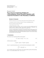
In Section 3 we present Quadrature methods used to completely determine the bifurcation
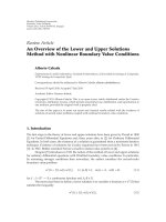
diagrams of 1.11 and 1.12 , respectively. We show that for β large enough, 1.10 has a
double S-shaped bifurcation curve with exactly 6 positive solutions for a certain range of λ
see Figure 1 .

2. Existence and Multiplicity Results when Ω is an
Annulus in Rn and n ≥ 1
Here we consider the existence of positive radial solutions for
−Δu
α x, u

∂u
∂η

λf u ,

Ω,

1 − α x, u u

2.1
0,

∂Ω,


4

Boundary Value Problems
103
102
ρ

101
100
10−1
10−2

0

1

2

3

4

5

6

λ

Figure 1: Double S-shaped bifurcation curve.

when f : 0, ∞ → 0, ∞ is a continuous function, Ω
and

{x ∈ Rn | R1 < |x| < R2 , 0 < R1 < R2 },

⎧
⎪0
⎨

if |x|

R1 ,

⎪ u

⎩
u 1

α u

if |x|

R2 .

2.2

Then the boundary condition of 2.1 is
0 if |x|

u
u

∂u
∂η

1

R1 ,

0 if |x|

2.3
R2 .

Thus to obtain positive solutions for 2.1 , we study

− Δu

in Ω,

λf u

2.4
u

0 on ∂Ω,

− Δu
u
∂u
∂η

in Ω,

λf u

0 if |x|

R1 ,

−1 if |x|

2.5
R2 .

The existence of positive solutions of 2.4 follows from 16, 18 in the following theorem.

Theorem 2.1 see 16, 18 . Assume (H1 ). Then 2.4 has a positive radial solution for all λ > 0.


Boundary Value Problems

5

Now we consider radial solutions to the problem 2.5 . Let
R2

−

m

R1

1
τ n−1

2.6

dτ.

R

By applying consecutive changes of variables, r |x|, s − r 2 1/τ n−1 dτ, t
and z t
u r
u |x| , 2.5 is equivalently transformed into the problem
λh t f z t

0 < t < 1,
−z t
−b,
z0
0,
z 1

m − s /m,

2.7

where
−mRn−1 > 0,
2

b

m2 r m 1 − t

ht

2 n−1

2.8
.

Note that h : 0, 1 → 0, ∞ is continuous function. For details about this transformation, see
19 . We prove the existence of a positive solution of 2.7 by using the fixed point index in a
cone. This fixed point index is equivalent to the Leray-Schauder degree which means that if
K is a cone in a Banach space E, O is bounded and open in E, 0 ∈ O, and T : K ∩ O → K is

completely continuous then
deg id − T ◦ r, r −1 K ∩ O , 0 ,

i T, K ∩ O, K

2.9

where r : E → K is an arbitrary retraction see 20 .
Lemma A see 21 . Let E be a Banach space, K a cone in E and O bounded open in E. Let 0 ∈ O,
and let T : K ∩ O → K be completely continuous. Suppose that T x / νx, for all x ∈ K ∩ ∂O and all
ν ≥ 1. Then
i T, K ∩ O, K

1.

2.10

Define Tλ : C 0, 1 → C 0, 1 by
Tλ z t

−bt

1

λ

G t, s h s f z s ds,

2.11

0

where

G t, s

⎧
⎨t,

0 ≤ t ≤ s ≤ 1,

⎩s,

0 ≤ s ≤ t ≤ 1.

2.12


6

Boundary Value Problems

Then Tλ : C 0, 1 → C 0, 1 is completely continuous and u is a solution of 2.7 if and only if u is
a fixed point of Tλ , that is, Tλ u u.
Theorem 2.2. If (H1 ) and (H2 ) both hold then 2.7
1
b/M 0 sh s ds, where b and h t are defined as in 2.8 .

has a positive solution for all λ >

Proof. Define K : {z ∈ C 0, 1 | z t ≥ 0, t ∈ 0, 1 and z is concave}, then K is a cone in
1
C 0, 1 . Further if λ > b/M 0 sh s ds, then Tλ K ⊂ K. In fact, if z ∈ K, then it is easy to show
that Tλ z 0

0 and Tλ z t ≤ 0 for t ∈ 0, 1 . Also if λ > b/M
Tλ z 1

−b

1
0

sh s ds, we have

1

λ

sh s f z s ds
0

≥ −b

2.13

1

λM

sh s ds > 0.
0

Thus Tλ z ∈ K.
Define f z : maxt∈ 0,z f t . Then f z ≤ f z , f is nondecreasing, and from H1 , we
have
lim

z→∞

Fix ρλ ∈ 0, 1/λ

1
0

f z
z

2.14

0.

sh s ds . From 2.14 , there is mλ > 0 such that
f z ≤ ρλ z ∀z ≥ mλ .

2.15

Let Oλ : {z ∈ C 0, 1 | z ∞ < mλ }. Then Oλ is bounded and open in C 0, 1 , 0 ∈ Oλ , and
Tλ : K ∩ Oλ → K is completely continuous. If z ∈ K ∩ ∂Oλ , then from monotonicity of f and
2.15 we have

Tλ z t ≤ λ

1

sh s f z s ds
0
1

≤ λf mλ

sh s ds
0

2.16

1

≤ λρλ mλ

sh s ds
0

< mλ

z

∞.

Thus Tλ z / νz for all ν ≥ 1. Now applying Lemma A, we have
i T λ , K ∩ Oλ , K

1,

which means that Tλ has a fixed point in K ∩ Oλ . Thus Theorem 2.2 is proven.

2.17


Boundary Value Problems

7

Further, if we additionally assume that
H3 N : supu∈ 0,∞ {f u } < ∞, then we can show nonexistence for λ
Theorem 2.3. If (H3 ) holds then 2.7 has no positive solution for all λ < b/N
and h t are defined as in 2.8 .

1.
1
0

sh s ds, where b

Proof. Suppose that uλ is a positive solution of 2.7 . Thus,
uλ t

−bt

T λ uλ t

1

G t, s h s f uλ s ds

λ
0

≤ −bt

2.18

1

G t, s h s ds.

λN
0

Letting t

1 gives
uλ 1 ≤ −b

1

sh s ds.

λN

2.19

0

Since uλ t is positive, we have
−b

1

λN

sh s ds ≥ 0

2.20

0

or, equivalently,
λ≥

b
N

1
0

sh s ds

.

2.21

Hence, the theorem is proved.
From Theorems 2.1 and 2.2, we have the following result.
Theorem 2.4. Assume (H1 ) and (H2 ). Then
1 if 0 < λ ≤ b/M

1
0

sh s ds, then 2.1 has a positive radial solution;

1

2 if λ > b/M 0 sh s ds, then 2.1 has at least two positive radial solutions, where b and
h t are defined as in 2.8 .

3. Existence of a Double S-Shaped Bifurcation Curve
3.1. A Quadrature Method for 1.11
In this section, we analyze the positive solutions when Ω
0, 1 , n 1, and f s
eβs/ β s .
The structure of positive solutions for 1.11 is well known for the case n
1, as well as


8

Boundary Value Problems
f u

eβ

u

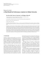
Figure 2: Graph of f u when β

2.

f u
eβ

u

μ0

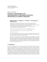
Figure 3: Graph of f u when β

5.

higher dimensions. It has been studied by authors such as those of 16, 22 , among others. For
completeness, we include the Quadrature method developed by Laetsch in 23 to analyze
positive solutions of the n 1 case, namely,
−u

λeβu/ β

u

: λf u ,

x ∈ 0, 1 ,

3.1

u 0

0,

3.2

u 1

0.

3.3

u

Define F u
f s ds, the primitive of f u . Figures 2 and 3 show f u plotted
0
for β 2 and β 5, respectively. Notice that f u is concave on 0, ∞ for β ∈ 0, 2 . When
β ∈ 2, ∞ , there exists a μ0 ∈ 0, ∞ such that f u is convex on 0, μ0 and concave on μ0 , ∞ .
For all β > 0, f u is increasing on 0, ∞ and bounded above by the horizonal asymptote,
y eβ . Also, F u is shown in Figure 4.
We present the main theorem of this subsection followed by computational results in
the form of bifurcation diagrams.
Theorem 3.1 see √ . Let β > 0, then 3.1 – 3.3 has a positive solution, u x , with u
16
√

ρ
2 0 ds/ F ρ − F s
λ for some λ > 0.
and only if G ρ :

∞

ρ if


Boundary Value Problems

9

F u

u

Figure 4: Graph of F u when β

5.

Proof. Fix β ∈ 0, ∞ . ⇒: Suppose that u x is a positive solution to 3.1 – 3.3 with u ∞ ρ.
First note that 3.1 is an autonomous differential equation. Thus, if there exists a x0 ∈ 0, 1
0 then both v x : u x0 x and w x : u x0 − x satisfy the initial value
such that u x0
problem,
−z

λf z ,

z0

u x0 ,

z 0

3.4

0

for all x ∈ 0, d where d min{x0 , 1 − x0 }. By Picard’s Existence and Uniqueness Theorem,
u x0 x ≡ u x0 −x . Hence, u x must be symmetric about x0 1/2 and u x ≥ 0; x ∈ 0, x0
while u x ≤ 0; x ∈ x0 , 1 . Now, multiplying 3.1 by u x yields,
−

2

u x
2

λ F u x

3.5

.

Integrating throughout 3.5 from x to 1/2, we have,
u x
F ρ −F u x

2λ,

x ∈ 0,

1
.
2

3.6

Integration of 3.6 from 0 to x gives
ux
0

Using the fact that u 1/2

ds
F ρ −F s

2λx,

x ∈ 0,

1
.
2

3.7

ρ, 3.7 becomes
G ρ :

√

ρ

2
0

ds
F ρ −F s

λ.

3.8


10

Boundary Value Problems

⇐: Suppose that there exists a λ, ρ ∈ 0, ∞ such that G ρ
0, 1/2 → R by
ux

ds

λ. Now, define u :

2λx.

F ρ −F s

0

√

3.9

We will show that u x is a positive solution of 3.1 . It follows that the left-hand side of 3.9
is a differentiable function of u which is strictly increasing from 0 to 1/2 as u increases from
0 to ρ. Hence, for each x ∈ 0, 1/2 , there exists a unique u x that satisfies
ux
0

ds

2λx.

F ρ −F s

3.10

By the Implicit Function Theorem, u x is differentiable as a function of x. Differentiating
3.10 , we have
2λ F ρ − F u x

u x

;

x ∈ 0,

1
.
2

3.11

Simplifying 3.11 gives
−

u x
2

2

λ F u x

−F ρ ;

−u x

x ∈ 0,

1
.
2

f ux .

3.12

Differentiating 3.12 , we have
3.13

Thus, u x satisfies the differential equation in 3.1 . Also, it is clear that u 0
0. Finally,
defining u x as a symmetric function on 0, 1 , gives a positive solution to 3.1 – 3.3 with
0 u 1.
u ∞ ρ and u 0
Remark 1 see 16 . G ρ is well defined and the included improper integral is convergent
since f ρ > 0 and F u is strictly increasing. Moreover, G ρ is a continuous and
differentiable function.
Also, analyzing 3.8 the following existence result was established in 16 .
Theorem 3.2 see 16 . For all β > 0, 1.11 has at least one positive solution for all λ > 0.

3.2. Computational Results for 1.11
In this subsection, we present the evolution of bifurcation curves for 1.11 suggested by our
computational results. Mathematica was employed to plot G ρ from Theorem 3.1 for various


Boundary Value Problems

11

103
102
ρ

101
100
10−1
10−2

0

1

2

3

4

5

6

7

λ

Figure 5: λ versus ρ for β

3.

values of β. Our results agree with those of previous authors such as 16 , who was first to
present them.

Case 1 see 16 . If β ∈ 0, β0
all λ > 0.

some β0 ≈ 4.25 then 1.11 has a unique positive solution for

Figure 5 gives a typical bifurcation diagram for β ∈ 0, β0 . Note that the following
figures are log plots.
Case 2 see 16 . If β ∈ β0 , ∞ then there exist λ0 , λ1 > 0 such that if
1 λ0 < λ < λ1 , then 1.11 has exactly 3 positive solutions;
2 λ

λ0 or λ

λ1 , then 1.11 has exactly 2 positive solutions;

3 0 < λ < λ0 or λ > λ1 , then 1.11 has a unique positive solution.
Figure 6 gives a typical bifurcation diagram for β ∈ β0 , ∞ .

3.3. A Quadrature Method for 1.12
We will adapt the Quadrature method to analyze solutions of 1.12 . Thus we study,
−u

λeβu/ β

u

: λf u ,

x ∈ 0, 1 ,

3.14

u 0

0,

3.15

u 1

−1,

3.16
u

where λ and β are positive parameters. Again, define F u
f s ds, the primitive of f u .
0
0
Using a similar argument to the one before, if there exists a x0 ∈ 0, 1 such that u x0
then u x is symmetric about x0 . Now, assume that u x is a positive solution of 3.14 – 3.16
0. Define q : u 1 . Clearly,
with ρ : u ∞ u x0 for some x0 ∈ 0, 1 such that u x0
u x ≥ 0 on 0, x0 and u x ≤ 0 on x0 , 1 . Hence, u x must resemble Figure 7.
λf u u . Integrating with respect to x gives
Multiplying 3.14 by u , we have −u u
−u
2

2

λF u

K.

3.17


12

Boundary Value Problems
103
102
ρ

101
100
10−1
10−2

λ0
0

λ1

1

2

3

4

5

6

7

λ

Figure 6: λ versus ρ for β

7.

ux

ρ
q

x

x0

1

Figure 7: Typical solution of 3.14 – 3.16 .

Substituting x x0 and x
−1 yields

u 1

1 into 3.17 while using u x0

−

F ρ
F q

1
2λ

F ρ

F q

K
,
λ
−

0, u x0

ρ, u 1

q, and

3.18

K

.
λ

3.19

1
.
2λ

3.20

Combining 3.18 and 3.19 gives

Substitution of 3.18 into 3.17 yields
− u
2

2

λ F u −F ρ .

3.21


Boundary Value Problems

13

Now, solving for u in 3.21 , we have
2λ F ρ − F u x

u x

x ∈ 0, x0 ,

,

3.22
− 2λ F ρ − F u x

u x

Integration of 3.22 combined with u 0
ux

ux

ds

We substitute x

− 2λ x − x0 ,

F ρ −F s

ρ

x0 into 3.23 and x

ds

ds

3.24

3.25

− 2λ 1 − x0 .

F ρ −F s

ρ

x ∈ x0 , 1 .

2λx0 ,

F ρ −F s

q

3.23

1 into 3.24 giving

ρ
0

x ∈ 0, x0 ,

2λx,

F ρ −F s

0

ρ gives,

0 and u x0

ds

x ∈ x0 , 1 .

,

3.26

Subtract 3.26 from 3.25 yields,
ρ

2
0

Solving 3.21 for

√

ds
F ρ −F s

2λ and using u 1

−

q
0

ds

2λ.

F ρ −F s

−1 and u 1

3.27

q, we have

1

2λ

F ρ −F q

.

3.28

Combining 3.28 with 3.27 we define,
ρ

H ρ, q : 2
0

ds
F ρ −F s

−

q
0

ds
F ρ −F s

−

1
F ρ −F q

.

3.29


14

Boundary Value Problems

Now, for each ρ ∈ 0, ∞ , we need to find a q q ρ ∈ 0, ρ such that H ρ, q ρ
fixed ρ ∈ 0, ∞ there is a unique q ρ ∈ 0, ρ with H ρ, q ρ
0 then
ρ

2
0

ds
F ρ −F s

−

q ρ

ds
F ρ −F s

0

1
F ρ −F q ρ

0. If for

2λ

3.30

will be satisfied for a unique λ ∈ 0, ∞ . As a result, we need to analyze the existence and
uniqueness of such a q q ρ . The following lemma lists several properties of H ρ, q .
Lemma B. 1 For every ρ > 0, H ρ, q → −∞ as q → ρ.
2 For all ρ > 0 and q ∈ 0, ρ one has that Hq ρ, q < 0.
3 H ρ, 0 → ∞ as ρ → ∞.
4 H ρ, 0 → −∞ as ρ → 0.
Proof. 1 It follows from the fact that F u is increasing and the Mean Value Theorem.
2 Fix ρ > 0. Then for all q ∈ 0, ρ ,

Hq ρ, q

−

1
F ρ −F q

−

f q
2 F ρ −F q

3/2

< 0.

3.31

3 For all ρ > 0,
ρ

H ρ, 0

ds

2

F ρ −F s

0

−

1
F ρ

3.32

⇒ H ρ, 0 → ∞ as ρ → ∞.
4 Again, this follows from the Mean Value Theorem and monotonicity of F u .
Notice that if H ρ, 0 > 0, then there will be a unique q ρ ∈ 0, ρ such that
H ρ, q ρ
0. From Lemma B, H ρ, q must resemble Figure 8.
Figures 9 and 10 show what H ρ, 0 resembles β ∈ 0, 4 and β ∈ 4, ∞ , respectively.
For β ∈ 0, 4 there exists a unique ρ0 > 0 such that if ρ ≥ ρ0 then H ρ, 0 ≥ 0 and if
ρ < ρ0 then H ρ, 0 < 0. In the second case, β ∈ 4, ∞ , the shape of H ρ, 0 changes from that
of the first case with the addition of both a local maximum and a local minimum. However,
based on our computations, we conjecture that there exists a unique ρ0 > 0 such that if ρ ≥ ρ0
then H ρ, 0 ≥ 0 and if ρ < ρ0 then H ρ, 0 < 0. Hence, for each ρ ∈ ρ0 , ∞ there is a unique
q ρ ∈ 0, ρ such that H ρ, q ρ
0. Next we define

H ρ, q ρ

:

1
2 F ρ −F q ρ

for all ρ ∈ ρ0 β , ∞ and q ρ ∈ 0, ρ and present the main theorem of the section.

3.33


Boundary Value Problems

15

H ρ, q

q

ρ
q ρ

Figure 8: Graph of H ρ, q .

H ρ, 0

ρ
ρ0

Figure 9: Graph of H ρ, 0 for β ∈ 0, 4 .

H ρ, 0

ρ1

ρ0

ρ

Figure 10: H ρ, 0 for β ∈ 4, ∞ .

Theorem 3.3. Let β > 0, then 3.14 – 3.16 has a positive solution, u x , with u ∞ ρ ∈ S β :
λ for some λ > 0 where q
q ρ ∈ 0, ρ is the unique solution of
ρ0 β , ∞ ⇔ H ρ, q ρ
H ρ, q ρ
0.
Proof. Fix β ∈ 0, ∞ . ⇒: is completed through preceding discussion.


16

Boundary Value Problems

⇐: Suppose that there exist λ ∈ 0, ∞ , ρ ∈ S β such that H ρ, q ρ
q ρ ∈ 0, ρ is the unique solution of H ρ, q ρ
0. Define u x : 0, 1 → R by
ux

ds
F ρ −F s

0

λ where

x ∈ 0, x0 ,

2λx,

3.34

ux

ds

− 2λ x − x0 ,

F ρ −F s

0

x ∈ x0 , 1 .

We will show that u x is a positive solution to 3.14 – 3.16 . Notice that the turning point of
u x , x0 , is given by
1
√
2λ

x0

ρ
0

ds
F ρ −F s

.

3.35

Clearly, for fixed λ,
1
√
2λ

ux

ds

3.36

F ρ −F s

0

is a differentiable function of u and is strictly increasing from 0 to x0 as u increases from 0 to
ρ. Hence, for each x ∈ 0, x0 there exists a unique u x such that

ux
0

ds

2λx.

F ρ −F s

3.37

By the Implicit Function Theorem, u x is differentiable with respect to x. This implies that,
2λ F ρ − F u x

u x

x ∈ 0, x0 .

,

3.38

A similar argument can be made to show that
u x

− 2λ F ρ − F u x

,

x ∈ x0 , 1 .

3.39

,

x ∈ 0, 1 .

3.40

From 3.38 and 3.39 , we have,
u x
2

2

λ F ρ −F u x


Boundary Value Problems

17

Differentiating 3.40 gives
λf u u ,

−u u
⇒ −u

x ∈ 0, 1 ,

λf u ,

x ∈ 0, 1 .

3.41

Hence, u x satisfies 3.14 . It only remains to show that u x satisfies 3.15 and 3.16 . But,
it is clear that u 0
0. Also, since H ρ, q ρ
λ, we have
1
F ρ −F q ρ

2λ

3.42

or equivalently,
1
.
2λ

F ρ −F q ρ
Substituting x

3.43

1 into 3.39 gives
− 2λ F ρ − F q ρ .

u 1

3.44

−1.

3.45

Combining 3.43 and 3.44 ,
u 1
Hence, u x satisfies both 3.15 and 3.16 .
To conclude the subsection, we present several results that detail the global behavior
of H ρ, q ρ .
Remark 1. Note that given β > 0, 3.14 – 3.16 has no positive solution with u

∞

< ρ0 β .

Remark 2. For every β > 0, H ρ, q ρ ≤ G ρ 2 for all ρ > ρ0 β . Moreover, equality is
0.
achieved if and only if ρ ρ0 β in which case, q ρ
This follows from observing that
H ρ, q ρ

1
2 F ρ −F q ρ
√
2

ρ
0

√
≤
2

ρ
0

ds

1
−√
F ρ −F s
2
ds
F ρ −F s

q ρ

ds
F ρ −F s

0

2

G ρ

2

.

2

3.46


18

Boundary Value Problems

Theorem 3.4. Let β > 0. If ρ ≥ ρ0 β , q ρ , and λ are as in the previous theorem with H ρ, q ρ
λ then
a q ρ → ρ as ρ → ∞, hence, x0 → 1 as ρ → ∞;
b λ → ∞ as ρ → ∞;
c λ ≥ 2ρ/e2β .
Proof. Fix β > 0 and let ρ ≥ ρ0 β , q ρ , and λ be as in the previous theorem with H ρ, q ρ
λ.
a Claim: ρ − q ρ ≤ eβ /4ρ
With this claim, it is clear that for fixed β, ρ − q ρ → 0 as ρ → ∞. Now to prove the
claim. Since H ρ, q ρ
λ, we have that
ρ

ρ

ds
F ρ −F s

0

dt
F ρ −F t

q ρ

1
F ρ −F q ρ

.

3.47

By the Mean Value Theorem, there exist θ1 ∈ s, ρ , θ2 ∈ t, ρ , and θ3 ∈ q ρ , ρ with s ∈
0, ρ and t ∈ q ρ , ρ such that
ρ

ds
√
f θ1 ρ − s

0

ρ

dt
ρ−t

f θ2

q ρ

1
f θ3

ρ−q ρ

.

3.48

Now, since f u is monotone increasing, we have that f θ1 , f θ2 ≤ f ρ and
1
f ρ

ρ
0

ds
√
ρ−s

1
f ρ

ρ

dt

≤
ρ−t

q ρ

1
f θ3

ρ−q ρ

.

3.49

.

3.50

A change of variables in the integrals of 3.49 yields,
√

ρ

1

f ρ

0

√

dv
1−v

√

ρ

f ρ

1
q/ρ

√

dw
1−w

1

≤
f θ3

ρ−q ρ

This implies that,

ρ−q ρ ≤

since f ρ ≤ eβ and f θ3 ≥ 1.

f ρ
eβ
≤
4f θ3 ρ 4ρ

3.51


Boundary Value Problems

19

103
102

ρ

101
100
ρ0
10−1
10−2

λ0
0

5

10

15

λ

Figure 11: Graph of λ versus ρ for β

2.

b By the Mean Value Theorem there exists a θ ∈ q ρ , ρ such that
λ

1
2f θ ρ − q ρ

.

3.52

But, 1 ≤ f θ ≤ eβ , which implies that
1
2eβ ρ − q ρ

≤λ≤

1
2 ρ−q ρ

.

3.53

Part a combined with 3.53 completes b .
c Finally 3.51 combined with 3.53 yields c .
Corollary 3.5. For every β > 0, there exists a λ1 > 0 such that 3.14 – 3.16 has no positive solution
for all λ < λ1 .

3.4. Computational Results for 1.12 and 1.10
This subsection will present computational results first for 1.12 then for our original
problem, 1.10 . In order to produce bifurcation diagrams, Mathematica was employed in
a two-step process. Recalling Theorem 3.3 from Section 3.3, for fixed β > 0 the corresponding
unique ρ0 β is first found using a standard root-finding algorithm. Then for each ρ ≥ ρ0 β ,
the same root-finding algorithm is employed to solve H ρ, q ρ
0 for the unique qvalue. Finally, H ρ, q ρ is evaluated for the given ρ and its unique q ρ to obtain the
corresponding unique λ. The result is a bifurcation diagram portraying λ versus ρ. Due to the
improper integrals in H ρ, q ρ , this procedure is computationally expensive. The numerical
investigations suggest the following evolution of bifurcation diagrams.
Case 1. For β ∈ 0, β1

for some β1 < 4 , there exists a λ0 > 0 such that if

1 λ ≥ λ0 , then 1.12 has a unique solution;
2 λ < λ0 , then 1.12 has no positive solution.
Figure 11 illustrates Case 1.


20

Boundary Value Problems

102

ρ

101
100
ρ0
10−1

λ1
0.5

λ0 λ2
1

1.5

2

2.5

λ

Figure 12: Graph of λ versus ρ for β

6.

Case 2. For β ∈ β1 , ∞ , there exists λ0 , λ1 , λ2 > 0 such that if
1 λ0 ≤ λ < λ2 , then 1.12 has exactly 3 positive solutions;
2 λ1 < λ < λ0 or λ

3 λ > λ2 or λ

λ2 , then 1.12 has exactly 2 positive solutions;

λ1 , then 1.12 has a unique positive solution.

Figure 12 shows a typical bifurcation diagram for Case 2.
u 1
0 and thus satisfies
Notice that λ0 , ρ0 corresponds to the case when q ρ
both 1.11 and 1.12 . We would then expect this to be the point at which the branch of
solutions of 1.10 bifurcates into the separate cases. To conclude the section, we present the
computational results for 1.10 by combining the solutions of 1.11 in Section 3.1 and 1.12
in Section 3.3.
Theorem 3.6. For β > 0, 1.10 has at least one positive solution for every λ > 0.
Case 1. For β ∈ 0, β1 , there exists a λ0 > 0 such that if
1 λ > λ0 , then 1.10 has 2 positive solutions,
2 λ ≤ λ0 , then 1.10 has a unique positive solution.
Figure 13 shows the complete bifurcation diagram of 1.10 for β

2.

Case 2. For β ∈ β1 , β0 , there exists λ0 , λ1 , λ2 > 0 such that if
1 λ0 < λ < λ2 , then 1.10 has exactly 4 positive solutions;
2 λ1 < λ ≤ λ0 or λ
3 λ > λ2 or λ

λ0 , λ2 , then 1.10 has exactly 3 positive solutions;

λ1 , then 1.10 has exactly 2 positive solutions;

4 λ < λ1 then 1.10 has a unique positive solution.
Case 2 is illustrated in Figure 14.
Case 3. For β ∈ β0 , β2

some β2 ∈ 6, 6.5 , there exists λi > 0 for i

0, 1, 2, 3, 4 such that if

1 λ0 < λ < λ2 or λ3 < λ < λ4 , then 1.10 has exactly 4 positive solutions;
2 λ1 < λ ≤ λ0 or λ

λ2 , λ3 , λ4 , then 1.10 has exactly 3 positive solutions;


Boundary Value Problems

21

103
102
ρ

101
100
10−1
10−2

λ0
0

1

2

3

4

5

6

5

6

λ
Dirchlet B.C.
Nonlinear B.C.

Figure 13: Graph of λ versus ρ for β

2.

103
102
ρ

101

100
10−1
10−2

λ1 λ0 λ2

0

1

2

3

4

λ
Dirchlet B.C.
Nonlinear B.C.

Figure 14: Graph of λ versus ρ for β

3 λ2 < λ < λ3 or λ > λ4 or λ

4.

λ1 , then 1.10 has exactly 2 positive solutions;

4 λ < λ1 , then 1.10 has a unique positive solution.
Case 3 is shown in Figure 15. Notice that the bifurcation diagram contains two Sshaped curves that do not overlap.

Case 4. For β ∈ β2 , ∞ , there exists λi > 0 for i

0, 1, 2, 3, 4 such that if

1 λ0 < λ < λ3 , then 1.10 has exactly 6 positive solutions;
2 λ2 < λ ≤ λ0 or λ

λ3 , then 1.10 has exactly 5 positive solutions;

3 λ3 < λ < λ4 or λ

λ2 , then 1.10 has exactly 4 positive solutions;

4 λ1 < λ < λ2 or λ

λ4 , then 1.10 has exactly 3 positive solutions;

5 λ > λ4 or λ

λ1 , then 1.10 has exactly 2 positive solutions;

6 λ < λ1 then 1.10 has a unique positive solution.


22

Boundary Value Problems
103
102
ρ

101
100
10−1
10−2

λ1

λ0 λ2

1

0

2

λ3
3

λ4
4

5

6

5

6

λ
Dirchlet B.C.
Nonlinear B.C.

Figure 15: Graph of λ versus ρ for β

5.

103
102
ρ

101
100
10−1 λ
1
10−2

λ2
0

λ0 λ3
1

2

λ4
3

4

λ
Dirchlet B.C.
Nonlinear B.C.

Figure 16: Graph of λ versus ρ for β

8.

Figure 16 exemplifies Case 4 with the complete bifurcation diagram for β 8. Again
the double S-shape appears but in this case the Ss overlap, yielding exactly 6 positive
solutions for a certain range of λ.

Acknowledgment
Eun Kyoung Lee was supported by the National Research Foundation of Korea Grant funded
by the Korean Government NRF-2009-353-C00042 .

References
1 R. S. Cantrell and C. Cosner, Spatial Ecology via Reaction-Diffusion Equations, Wiley Series in
Mathematical and Computational Biology, John Wiley & Sons, Chichester, UK, 2003.
2 R. S. Cantrell and C. Cosner, “Density dependent behavior at habitat boundaries and the Allee effect,”
Bulletin of Mathematical Biology, vol. 69, no. 7, pp. 2339–2360, 2007.


Boundary Value Problems

23

3 R. S. Cantrell, C. Cosner, and S. Mart´nez, “Global bifurcation of solutions to diffusive logistic
ı

equations on bounded domains subject to nonlinear boundary conditions,” Proceedings of the Royal
Society of Edinburgh. Section A, vol. 139, no. 1, pp. 45–56, 2009.
4 J. Goddard II and R. Shivaji, “A population model with nonlinear boundary conditions and constant
yield harvesting,” submitted.
5 J. Bebernes and D. Eberly, Mathematical Problems from Combustion Theory, vol. 83 of Applied
Mathematical Sciences, Springer, New York, NY, USA, 1989.
6 Y. Du and Y. Lou, “Proof of a conjecture for the perturbed Gelfand equation from combustion theory,”
Journal of Differential Equations, vol. 173, no. 2, pp. 213–230, 2001.
7 S. P. Hastings and J. B. McLeod, “The number of solutions to an equation from catalysis,” Proceedings
of the Royal Society of Edinburgh. Section A, vol. 101, no. 1-2, pp. 15–30, 1985.
8 P. Korman and Y. Li, “On the exactness of an S-shaped bifurcation curve,” Proceedings of the American
Mathematical Society, vol. 127, no. 4, pp. 1011–1020, 1999.
9 P. Korman and J. Shi, “Instability and exact multiplicity of solutions of semilinear equations,” in
Proceedings of the Conference on Nonlinear Differential Equations (Coral Gables, FL, 1999), vol. 5 of
Electronic Journal of Differential Equations Conference, pp. 311–322, Southwest Texas State University,
San Marcos, Tex, USA.
10 J. R. Parks, “Criticality criteria for various configurations of a self-heating chemical as functions of
activation energy and temperature of assembly,” The Journal of Chemical Physics, vol. 34, no. 1, pp.
46–50, 1961.
11 S. V. Parter, “Solutions of a differential equation arising in chemical reactor processes,” SIAM Journal
on Applied Mathematics, vol. 26, pp. 687–716, 1974.
12 D. H. Sattinger, “A nonlinear parabolic system in the theory of combustion,” Quarterly of Applied
Mathematics, vol. 33, pp. 47–61, 1975/76.
13 K. K. Tam, “Construction of upper and lower solutions for a problem in combustion theory,” Journal
of Mathematical Analysis and Applications, vol. 69, no. 1, pp. 131–145, 1979.
14 S. H. Wang, “On S-shaped bifurcation curves,” Nonlinear Analysis: Theory, Methods & Applications, vol.
22, no. 12, pp. 1475–1485, 1994.
15 S.-H. Wang and T.-S. Yeh, “Exact multiplicity of solutions and S-shaped bifurcation curves for the
p-Laplacian perturbed Gelfand problem in one space variable,” Journal of Mathematical Analysis and
Applications, vol. 342, no. 2, pp. 1175–1191, 2008.

16 K. J. Brown, M. M. A. Ibrahim, and R. Shivaji, “S-shaped bifurcation curves,” Nonlinear Analysis:
Theory, Methods & Applications, vol. 5, no. 5, pp. 475–486, 1981.
17 R. Shivaji, “A remark on the existence of three solutions via sub-super solutions,” in Nonlinear Analysis
and Applications (Arlington, Tex., 1986), vol. 109 of Lecture Notes in Pure and Applied Mathematics, pp.
561–566, Dekker, New York, NY, USA, 1987.
18 H. Wang, “On the existence of positive solutions for semilinear elliptic equations in the annulus,”
Journal of Differential Equations, vol. 109, no. 1, pp. 1–7, 1994.
19 Y.-H. Lee, “Multiplicity of positive radial solutions for multiparameter semilinear elliptic systems on
an annulus,” Journal of Differential Equations, vol. 174, no. 2, pp. 420–441, 2001.
20 H. Amann, “Fixed point equations and nonlinear eigenvalue problems in ordered Banach spaces,”
SIAM Review, vol. 18, no. 4, pp. 620–709, 1976.
21 D. J. Guo and V. Lakshmikantham, Nonlinear Problems in Abstract Cones, Academic Press, Orlando,
Fla, USA, 1998.
22 A. Castro and R. Shivaji, “Nonnegative solutions for a class of nonpositone problems,” Proceedings of
the Royal Society of Edinburgh. Section A, vol. 108, no. 3-4, pp. 291–302, 1988.
23 T. Laetsch, “The number of solutions of a nonlinear two point boundary value problem,” Indiana
University Mathematics Journal, vol. 20, pp. 1–13, 1970.