Tax revenue, expenditure, and economic growth: An analysis of long-run relationships

4

Nguyen Phuong Lien & Su Dinh Thanh / Journal of Economic Development 24(3), 04-26



Tax revenue, expenditure, and economic growth:
An analysis of long-run relationships
NGUYEN PHUONG LIEN
Hoa Sen University –
SU DINH THANH
University of Economics HCMC –

ARTICLE INFO

ABSTRACT

Article history:

Focusing on the investigation of “long-term” relationship between tax
revenue, expenditure, and economic growth, this paper employs the
Granger causality test and finds that the linkage between tax revenue
and spending is a bi-directional causal correlation. Furthermore,
applying Persyn and Westerlund’s (2008) co-integration test allows
for corroboration of existence of long-run cointegration linkages
among outcome of economy and the three variables. In addition, by
adopting two-step system generalized method of moments (SGMM)
for a dynamic panel of 82 developed and developing countries during
16-year period (2000–2015), this research demonstrates that the
impact of tax revenue and spending is substantial and ambiguous,

depending on different groups of economies.

Received:
Dec., 23, 2016
Received in revised form:
May, 15, 2017
Accepted:
June, 30, 2017
Keywords:
long-term economic
growth, co-integration
test, tax revenue and
expenditure.



Nguyen Phuong Lien & Su Dinh Thanh / Journal of Economic Development 24(3), 04-26

5



1. Introduction
It is widely known that any change in
public policy can affect economic activities
(Holley, 2011). During the last decades there
have been numerous studies that
investigated the linkage between public
spending or tax revenue and economic
growth. Dzhumashev (2014) revealed that

relations among public finance, institutional
quality, and economic growth are too
ambiguous, which needs to be clarified.
Furthermore, despite Barro’s (1990)
argument that it is equal to public
expenditure, tax revenue depends on public
expenses. The question, therefore, is “how
does tax revenue correlate closely with
government expenditure?” In the past two
decades, the results seem to be mixed and
confusing.
In addition, through the statistics
obtained of income per capita, tax revenue,
and government expenditure, this research
shows different trends of these variables by
types of economic groups. While developed
countries are likely to collect more taxes,
spend less, and maintain the slow speed of
growing outcome, developing countries
keep spending more and collect less revenue
for rapid growth in their economies (see
appendix A). Moreover, a marked difference
between developed and developing
countries lies in the fact that developing
countries constitute more than 60% of the
world population, but they contribute less
than 30% to global GDP (Spence, 2011).
This paper initially attempts to
investigate the causal correlation between

tax revenue and government spending. The
second objective is to evaluate long-run
economic growth affected by tax revenue
and government expenditure (hereafter
termed “public finance factors”). Finally, it
is imperative to estimate the level effects of
tax revenue and expenditure on economic
growth depending on kinds of groups of
economies to expand the literature on
endogenous economic growth.
Besides the introduction, this paper is
structured as follows. The second section
discusses the theoretical background and
briefly describes previous research findings
in the same field. Section 3 presents the
empirical dataset and findings, followed by
Section 4, which concludes the study and
also draws a few implications.

2. Theoretical
bases,
previous
empirical
research,
and
methodologies
Relationship between tax revenue and
government spending
The interaction between tax revenue and
government spending can be divided into

three strands. First, there is a fiscal
synchronization hypothesis that confirms
the bidirectional causal link between the two
variables (Musgrave, 1966; Meltzer &
Richard, 1981; Bohn, 1991; Chang &
Chiang, 2009). Second, the “spend-tax”
hypothesis,
which
maintains
that
government expenditure can be a root cause
of change in tax revenue (Friedman, 1978;
Darrat, 1998; Blackley, 1986). The last
strand is reflected through “tax-spend”
hypothesis that takes into account the role of



6

Nguyen Phuong Lien & Su Dinh Thanh / Journal of Economic Development 24(3), 04-26

tax revenue in enabling government to lead
expenses (Mahdavi & Westerlund, 2008;
Hansan et al., 2012). However, most studies
examined panel data of high income
countries or of merely one country and
arrived at main conclusions to justify the
three listed hypotheses. For supporting
government planners, a question can be

posed as to whether there exists a
bidirectional causality linkage between tax
revenue and expenditure for both developed
and developing countries.
To investigate this relationship, this
study applies the causality theory suggested
by Granger (1969) and sets out to examine
the bidirectional causal linkage between tax
revenue and government spending in the
context of developed and developing
countries. The null hypothesis can be
formulated as follows:
(()

𝐻" :𝛽&
(()

𝐻- : 𝛽&

= 𝛽 (() ∀&,-,……0 , ∀(,-,….,2
(

≠ 𝛽4 , 𝑘 ∈ 1, … . , 𝑝 , ∃ 𝑖, 𝑗
∈ 1, … . , 𝑁

𝑆𝑅𝑅( − 𝑆𝑅𝑅- /𝑝(𝑁 − 1)

𝑆𝑅𝑅- / 𝑁𝑇 − 𝑁 1 + 𝑝 − 𝑝

The empirical research equation for

Granger test is computed as:
𝑡𝑎𝑥𝑟𝑒𝑣&,J = 𝛽" +


2
&,- 𝛿- 𝑡𝑎𝑥𝑟𝑒𝑣&,JL-

𝑔𝑒𝑥𝑝&,J = 𝛾" +


2
&,- 𝜃- 𝑔𝑒𝑥𝑝&,JL-

(
&," 𝛽- 𝑔𝑒𝑥𝑝&,JL-

+ 𝜀& + 𝜗&,J
(
&," 𝛾- 𝑡𝑎𝑥𝑟𝑒𝑣&,JL-

+ 𝜀& + 𝜗&,J

where 𝑡𝑎𝑥𝑟𝑒𝑣&,J is the proportion of total tax
revenue to gross domestic products (GDP)
of country i (i=1,…N) at time t (t=1,…T),
𝑔𝑒𝑥𝑝&,J denotes the proportion of total
government expenditure to GDP, k and p
are latencies, 𝜀& stands for countrycharacteristic effects, and 𝜗&,J represents the
observation error with E(𝜗&,J ) = 0.
In addition, short-term tax changes can

be different from long-run effects because of
a great elasticity of demand curve (Holley,
2011). In the past decade there have been
few studies performing a comprehensive
analysis of this difference to help policy
makers design the appropriate policies in
public finance.
Since it helps avoid the bias given the
case of regressions from nonstationary
variables, multiple studies employed cointegration test to clear up the problem of
spurious regression (e.g., McCoskey & Kao,
1999; Bai & Ng, 2004; Pedroni, 2004;
Breitung & Pesaran, 2005; Westerlund &
Edgerton, 2008; Persyn & Westerlund,
2008).
The following question, therefore, should
be
determined:
“Do
cointegration
relationships exist among tax revenue,
government spending, and long-run
economic growth?”

The corresponding F test is:
𝑍=



+

(1)
+

(2)

In addition, the error-correction (EC)
model is often applied to investigate the
long-run relationship between stationary as
well as cointegrated variables (Ojede &
Yamarik, 2012).
Assuming that i represents a country and
t is time period, the long-run relationship can
be represented as below:



Nguyen Phuong Lien & Su Dinh Thanh / Journal of Economic Development 24(3), 04-26

7


V
𝑙𝑟𝑔𝑑𝑝&,J = 𝛼",& + 𝛼&,J
𝑋&,J + 𝑢&,J ,

(3)

where 𝑙𝑟𝑔𝑑𝑝&,J is logarithm of real GDP per
capita (dependent variable), 𝛼",& is a

V
country-specific intercept term, 𝛼&,J
denotes

country-characteristic slope coefficients, X
indicates the vector of public finance and
institutional quality, and 𝑢&,J is an error term
of country i at time t.
In case a co-integration linkage exists
between 𝑙𝑟𝑔𝑑𝑝&,J and X variables, and error
term 𝑢&,J is an I(0) process for all countries
i, we can re-write the growth equation in
terms of an autoregressive distributed lag
(ARDL) of order (p,q) as below:
𝑙𝑟𝑔𝑑𝑝&,J = 𝛽-,& 𝑙𝑟𝑔𝑑𝑝&,JL- +
𝛽Z,& 𝑙𝑟𝑔𝑑𝑝&,JLZ + ⋯ + 𝛽2,\ 𝑙𝑟𝑔𝑑𝑝&,JL2 +
V
V
V
𝜎",&
𝑋&,J + 𝜎-,&
𝑋&,JL- + ⋯ + 𝜎^,&
𝑋&,JL^ +

𝜀& + 𝜗&,J ,

(3a)

where p is number of lag of dependent
variable, and q is number of lag of

independent variables.
Then, we re-design the error-correction
model as follows:
∆𝑙𝑟𝑔𝑑𝑝&,J =
^L- V
4," 𝜎4,& ∆𝑋&,JL4
V
𝜃-,& 𝑋&,J + 𝜗&,J

2L4,- 𝛽4,& ∆𝑙𝑟𝑔𝑑𝑝&,JL4

+

+ 𝜇& 𝑙𝑟𝑔𝑑𝑝&,JL- − 𝜃",& −

(3b)

where 𝛽4,& and 𝜎4,J are short-run coefficients,
𝜃",& and 𝜃-,& stand for long-run coefficients,
and 𝜇& represents an adjustment-speed
(error-correction term) to the long-run
equilibrium.
Definition of public finance and its effect
on economic growth

As documented by Barro (1990),
Buchanan (1999), Wellisch (2004), Kaul
and Conceição (2006), and McGee (2013),
tax revenue and expenditure are two major
components of public finance. Barro (1990)

explained the mode of interaction between
government expenditure and taxes with their
effects on household spending and income.
Moreover, from Barro’s (1990) perspective,
there might be a too simple social regime,
where government collects taxes from
income and property only. The limitation of
this research is that it does not evaluate the
relationship between total tax revenue and
total public spending, which articulates the
government capability.
In the last decades, two stances have
emerged in evaluating growth effect of tax
revenue and government expenditure. First,
a number of researchers used the
endogenous growth model to estimate the
impact of tax revenue or expenditure in
isolation. Second, they applied the causality
or cointegration test to capture the linkage
between economic growth and tax structure
or share of expenditure.
A few previous investigations indicated
that income tax, sale tax, or property tax has
full meaning in reducing economic outcome
in both developing and developed
economies (Lee & Gordon, 2005; Ojede &
Yamarik, 2012; Amir et al., 2013, Adkisson
& Mohammed, 2014). In addition, Bujang et
al. (2013) employed Kao’s cointegration test
for a panel dataset of 24 developing and 24

developed countries in a 10-year period and
mentioned that tax structure and GDP in
developing countries do not have the longrun cointegrating linkages, but only in



8

Nguyen Phuong Lien & Su Dinh Thanh / Journal of Economic Development 24(3), 04-26

developed countries do these links exist.
Furthermore, Easterly and Rebelo (1993)
revealed that income tax increases economic
growth, while custom tax reduces it.
Some earlier studies also showed the
mixed growth effect of government
spending and tax revenue. Barro (1991)
performed an empirical study of 98
countries from 1960 to 1985 and noted that
the relationship between public spending
and economic growth is negative.
Furthermore, Hitiris and Posnett (1992)
analyzed the data of 20 OECD countries
over a 28-year period, demonstrating that
when government spends a certain amount
on health care, this expense can promote
income per capita. Applying OLS, fix
effects, and pooled OLS techniques, Kneller
et al. (1999) performed an analysis of the
dataset of 22 developed countries between

1970 and 1995 and found that government
spending positively affects income per
capita, whilst taxation exerts a harmful
effect on this variable. Cooray (2009)
adopted the generalized method of moments
to indicate that public spending and quality
of governance positively affect economic
growth. In addition, Dzhumashev (2014)
argued that public expenditure depends on
effectiveness of governance as well as level
of corruption. How do tax revenue and
expenditure afftect economic growth? Do
their levels of effects differ considering
different kinds of economic groups? The
questions are to be tackled in the next
sections of this study.
Methodologies
Before running co-integration test, this
paper employs the unit root test following



HT (1999) and IPS (2003). The HarrisTzavalis (HT) (1999) test hypothesizes that
all panels have the same autoregressive
parameter and rho is smaller than 1. It also
assumes that the periods of time are fixed,
which is similar to the Levin-Lin-Chu test.
However, the IPS test does not necessitate
balanced data, but requires that T must be at
least 5, if the dataset is strongly balanced for

the asymptotic normal distribution of Z-ttilde-bar to hold.
For co-integration test, this study follows
Persyn and Westerlund’s (2008) proposed
technique, developed by Westerlund (2007).
This allows for complete check of
heterogeneous characteristics of long-run
parts of error correction model. The null
hypothesis is H0: ai = 0 for all i, (i= 1,…N)
and H1: : ai < 0 for all I, (i= 1,…N). This test
uses the Ga and Gt test statistics for checking
the null hypothesis for at least one i. These
statistics start from a weighted average of
the individually estimated ai's and their tratio’s respectively. The test also requires
that the null hypothesis (H0) be rejected for
accumulating evidence of co-integration of
at least one of the cross-sectional units. The
Pa and Pt test statistics pool information over
all the cross-sectional units to test H0: ai = 0
for all i, (i= 1,…N) and H1: : ai < 0 for all I,
(i= 1,…N). Rejection of H0 is thus
substantial to validate existence of cointegration given the entire panel.
After identifying the co-integration
linkages
between
dependent
and
independent variables, this paper adopts the
two-step system generalized method of
moments (SGMM) method for a dynamic
panel of the whole sample as well as for

9

Nguyen Phuong Lien & Su Dinh Thanh / Journal of Economic Development 24(3), 04-26


cluster data to determine the levels of effects
of tax revenue and government expenditure
on economic growth in both developed and
developing countries. According to the
numerous previous studies, this technique
can help achieve more consistent
endogenous growth model than fixed effects
method (Arrellano & Bond, 1991; Baltagi,
2005; d’Agostino et al., 2012; Sasaki, 2015).
Furthermore, endogenous variables always
appear in growth models, which causes bias
to OLS regression, and using exogenous
instruments could help regressors fix this
issue (Barro 1990; Acemoglu et al., 2001).
Siddiqui and Ahmed (2013) indicated that
generalized method of moments (GMM) is
an instrumental technique, which handles
the endogenous phenomenon as well as the
matter of inefficiency in the presence of
heteroskedasticity. Owing to the bias of the
lagged dependent variable in the right-handside, the first-different GMM helps
regressors elimilate the bias of fixed effects

and unobserved error term effects
(Arellanon & Bond, 1991; Roodman, 2009).
In addition, Windmeijer (2005) revealed that
the two-step GMM procedure obtains
consistent and efficient parameters of
estimation. This study, therefore, applies
two-step SGMM to the dynamic panel data
of 38 developed and 44 developing countries
in a 16-year period.
In accordance with Barro (1990) and
Barro and Sala-i-Martin (1992), the

empirical model for estimating degrees of
effects of tax revenue and government
expenditure on economic growth are as
below:
𝑙𝑟𝑔𝑑𝑝&,J = 𝛼" + 𝛼- 𝑙𝑟𝑔𝑑𝑝&,JL- +
𝛼Z 𝑡𝑎𝑥𝑟𝑒𝑣&,J + 𝛼c 𝑖𝑛𝑓𝑙&,J + 𝛼f 𝑡𝑟𝑎𝑑𝑒𝑜𝑝&,J +
𝛼h 𝑡𝑖𝑛𝑣&,J + 𝛼i 𝑡𝑜𝑝𝑜𝑝&,J + 𝛼j ℎ𝑑𝑖&,J + 𝜀&,J +
𝜗&,J

(4a)

𝑙𝑟𝑔𝑑𝑝&,J = 𝛼" + 𝛼- 𝑙𝑟𝑔𝑑𝑝&,JL- +
𝛼Z 𝑔𝑒𝑥𝑝&,J + 𝛼c 𝑖𝑛𝑓𝑙&,J + 𝛼f 𝑡𝑟𝑎𝑑𝑒𝑜𝑝&,J +
𝛼h 𝑡𝑖𝑛𝑣&,J + 𝛼i 𝑡𝑜𝑝𝑜𝑝&,J + 𝛼j ℎ𝑑𝑖&,J + 𝜀&,J +
𝜗&,J ,

(4b)

where, 𝑖𝑛𝑓𝑙&,J is Inflation of country i
(i=1,…N) at time t (t=1,…T), 𝑡𝑟𝑎𝑑𝑒𝑜𝑝&,J
stands for trade openness, 𝑡𝑖𝑛𝑣&,J represents
total

investment,

𝑡𝑜𝑝𝑜𝑝&,J

is

total

population,
and
ℎ𝑑𝑖&,J
is
human
development index, surveyed and measured
by United Nations Development Program
(UNDP).

3. Empirical data and findings
We extract the annual data for the whole
sample, which includes 38 developed and 44
developing countries over a 16-year period
(2000–2015) (see Appendix B—List of
studied countries), and the strong balanced
panel data is used for analysis (see Table 1—
Description of variables).

10

Nguyen Phuong Lien & Su Dinh Thanh / Journal of Economic Development 24(3), 04-26



Table 1
Description of variables (for the whole sample of 82 developed and developing
countries)
Meaning and source

Variable

Obs.

Mean

Std. dev.

Min

Max

Real gross domestic per
capita (US dollars) –
world bank website
(WB) (updated on

August 10, 2016)

rgdp

1312

16,948.350

19,550.880

194.169

91,593.630

Total tax revenue (% of
GDP) – International
Monetary Fund (IMF)
(updated in April 2016)

taxrev

1312

30.561

11.522

8.489

57.435

Total
government
expenditure (% of
GDP) – (IMF) (updated
in April 2016)

gexp

1312

32.731

11.519

10.529

65.572

Inflation(Consumer
annual Price index) –
(WB)

infl

1312

5.199

7.550

-8.238

168.620

Trade (% of GDP) –
(WB)

tradeop

1312

82.488

57.468

4.692

439.657

Total
domestic
investment (% of GDP)
– (IMF) (updated in
April 2016)

tinv

1312

23.586

5.981

8.675

58.151

Total
population
(People) – (WB)

topop

1312

5E+07

1.4E+08

81,131

1.3E+09

Human
development
index (index) – United
Nations development
program (UNDP)

hdi

1312

0.727

0.150

0.283

0.949

Table 1 shows the big gap between developed and developing countries in real GDP per
capita, tax revenue, and expenditure.



11

Nguyen Phuong Lien & Su Dinh Thanh / Journal of Economic Development 24(3), 04-26



Table 2
Correlation matrix (for the whole sample of 82 developed and developing countries)
lrgdp
lrgdp

1

taxrev

0.745***

taxrev

gexp

infl

tradeop

tinv

topop

hdi

1

0.000
gexp

infl

tradeop

tinv

topop

hdi

0.695***

0.933***

0.000

0.000

-0.279***

-0.176***

-0.189***

0.000

0.000

0.000

0.137***

0.104***

0.059*

-0.017

0.000

0.000

0.034

0.536

-0.036

-0.010

-0.068**

0.174***

0.164***

0.195

0.705

0.015

0.000

0.000

-0.155***

-0.193***

-0.136***

0.069**

-0.202***

0.155***

0.000

0.000

0.000

0.013

0.000

0.000

0.862***

0.697***

0.679***

-0.189***

0.142***

0.050*

-0.133***

0.000

0.000

0.000

0.000

0.000

0.068

0.000

1

1

1

1

1

Note: *p < 0.1, **p < 0.05, ***p < 0.01

Through Table 2, it can be observed that tax revenue and expenditure are significantly
and strongly correlated with economic growth and that tax revenue and expenditure are
closely correlated with each other.

1



12

Nguyen Phuong Lien & Su Dinh Thanh / Journal of Economic Development 24(3), 04-26



Table 3a
Results of unit root test for a panel with normal data for the whole sample in 2000–
2015
Normal

HT test

IPS test

rho Statistic

z

p-value

Statistic

p-value

AIC chosen lags
average

rgdp

0.904

4.000

1.000

8.270

1.000

0.45

lrgdp

0.935

5.544

1.000

3.136

0.999

0.45

taxrev

0.4871***

-16.778

0.000

-3.679***

0.000

0.50

gexp

0.618***

-10.266

0.000

-4.008***

0.000

0.48

hdi

0.908

4.191

1.000

-0.458

0.324

0.51

infl

0.331***

-24.551

0.000

-12.643***

0.000

0.34

0.794

-1.478

0.0697

-1.981**

0.023

0.65

0.715***

-5.414

0.000

-1.789**

0.0368

0.41

0.989

8.267

1.000

7.724

1.000

1.50

0.000

1.540

tradeop
tinv
topop
ltopop

0.342

***

-20.241

0.000

-3.557

***

Note: *p < 0.1, **p < 0.05, ***p < 0.01

The table shows three variables that do not stay significant, including “real income per
capita,” “human development indicator,” and “total population.” This finding is underpinned
by Bujang et al. (2013), which demands identification of co-integration linkages between
non-stationary variables and others.
This study continues by running the unit root test for first different values of variables,
noting that all variables stay significant at first differences concerning both HT and IPS test.
The variable “total population” is significant after taking the first difference of logarithm
using IPS test.



13

Nguyen Phuong Lien & Su Dinh Thanh / Journal of Economic Development 24(3), 04-26



Table 3b
Results of unit root test for a panel with data of first different values for the whole sample
in 2000–2015
First difference

HT test
rho
Statistic

IPS test

z

p-value

Statistic

p-value

AIC
chosen lags
average

∆.rgdp

0.263***

-25.835

0.000

-12.688***

0.000

0.43

∆.lrgdp

0.295***

-24.326

0.000

-12.517***

0.000

0.39

∆.taxrev

-0.251***

-50.038

0.000

-22.404***

0.000

0.37

∆.gexp

-0.093***

-42.598

0.000

-22.405***

0.000

0.32

∆.hdi

0.194***

-29.074

0.000

-14.013***

0.000

0.23

∆.infl

-0.071***

-41.564

0.000

-31.341***

0.000

0.76

∆.tradeop

-0.114***

-43.586

0.000

-20.248***

0.000

0.38

∆.tinv

-0.110***

-43.375

0.000

-21.673***

0.000

0.41

∆.topop

0.591***

-10.413

0.000

2.045***

0.980

1.37

∆.ltopop

0.366***

-20.993

0.000

-6.039***

0.000

1.28

Note: *p < 0.1, **p < 0.05, ***p < 0.01

Tables 3a and 3b show the evidence of stationarity for all variables; it means that a unit
root is absent from the error term in the panel dataset.

Table 4
Pairwise Granger test results
H0: Government expenditure does not Granger cause tax
revenue (dependent variable: taxrev)

Obs.

z-Stat

Prob.

gexpà taxrev

1312

36.71***

0.000

1312

36.12***

0.000

H0: Tax revenue does not Granger cause government
expenditure (dependent variable: gexp)
taxrevà gexp
Note: *p < 0.1, **p < 0.05, ***p < 0.01



14

Nguyen Phuong Lien & Su Dinh Thanh / Journal of Economic Development 24(3), 04-26



Table 5
Westerlund long-run cointegration test: Dependent variable: lrgdp (Average AIC
selected lag length: 1)
taxrev - lrgdp
Statistic

gexp - lrgdp

Value

Z-value

P-value

Gt

-3.357***

-11.281

Ga

-20.018***

infl - lrgdp

Value

Z-value

P-value

0.000

-2.610***

-2.863

-11.055

0.000

-19.169***

Pt

-22.008

***

-3.349

0.000

Pa

-14.012***

-7.668

0.000

AIC lead length:

0.55

Value

Z-value

P-value

0.002

-3.425***

-12.050

0.000

-9.898

0.000

-20.294***

-11.430

0.000

-16.047

3.594

1.000

-17.625

1.755

0.960

-9.865*

-1.381

0.084

-12.605***

-5.536

0.000

0.63

tradeop - lrgdp
Statistic

Value
-2.801***

Gt
Ga

-18.042

Pt

-19.057

Pa

-12.740

***

***

AIC lead length:

0.63
tinv - lrgdp

Z-value

P-value

-5.020

0.000

Value

Z-value

P-value

-3.610***

-14.141

0.000

***

-8.364

0.000

-19.987

0.087

0.535

-21.637***

0.000

***

-5.739
0.71

hdi - lrgdp

-16.441
0.74

Value

Z-value

P-value

-3.968***

-18.175

0.000

***

-6.817

0.000

-11.012

0.000

-16.905

-2.917

0.002

-24.096***

-5.782

0.000

0.000

***

-8.567

0.000

-11.351

-14.605
0.63

topop - lrgdp
Statistic

Value

Z-value

P-value

Gt

-4.912***

-11.281

0.000

Ga

-13.336***

-11.055

0.000

Pt

-24.764

***

-3.349

0.000

Pa

-10.743***

-7.668

0.000

AIC lead length:
*

0.71
**

Note: p < 0.1, p < 0.05, ***p < 0.01
Table 4 indicates that there exists a bidirectional and causal relationship between
tax revenue and government, which supports
the fiscal synchronization hypothesis that is
justified by a few previous studies such as
Musgrave (1966), Meltzer and Richard
(1981), Bohn (1991), and Chang and Chiang
(2009). This result also suggests that policy

makers in both developed and developing
countries should focus on the important role
of total tax revenue and expenditure for
larger government budget as well as
increasing economic outcomes to develop
appropriate fiscal synchronization in these
economies.
Before performing regression analysis of



Nguyen Phuong Lien & Su Dinh Thanh / Journal of Economic Development 24(3), 04-26

15


the level effects of tax revenue, expenditure,
and economic growth, this research employs
co-integration test to avoid bias from nonstationary variables and answer the second
research question: “Do co-integration

relationships exist among tax revenue,
government spending, and long-run
econmic growth?”
Co-integration test results:
H0: In each pair of variables there exists
no long-term co-integration linkageThe cointegration test results indicate that the
linkages between tax revenue or expenditure
and economic growth are co-integrated.
Interestingly, this finding supports not only
the line trend graphs discussed earlier (see
Appendix A) but also the fiscal
synchronization hypothesis confirmed by
Chang and Chiang (2009) for the case of 15
OECD countries over the 1992–2006 period.
Furthermore, to overcome the limitation
of previous studies that run causality or cointegration test for investigating the
correlations
among
tax
revenue,
expenditure, and long-run economic growth,
this research also seeks to determine the
degrees of effects of these two variables on
economic growth.
In light of the bias caused by the dynamic
characteristic of strong balanced panel data
of 82 countries in a 16-year period, this
research applies the two-step system

generalized method of moments (SGMM) to

estimate the level effects of tax revenue and
expenditure on economic growth (Baltagi,
2005.) Roodman (2009) noted that SGMM
estimation
typically
includes
more
instruments, which therefore increases the
efficiency of the regression. To apply the
SGMM estimation we conduct the Hansen
test of over-identifying restrictions to check
the null hypothesis that the instrumental
variables are exogenous. If the null
hypothesis can be rejected, then the SGMM
estimation can fix the problem of
endogeneity, and the regression will provide
results with small bias. In the case of “large
N and small T,” the Hansen test is
appropriate to verify the endogenous
phenomenon (Hansen, 1982; Baltagi, 2005).
Using dynamic panel data always
encounters autocorrelation problems. For
this reason we employ Arellano–Bond test
to identify the autocorrelation of different
error terms; it involves E (∆𝑈&J , ∆𝑈&JLZ = 0)
(Arellano & Bond, 1991). We also apply two
types of unit root test to identify stationary
variables before running SGMM for
reducing bias from time series data in longrun period. Most variables stay significant at
first lag or first differences given HT and

IPS unit root tests (see Tables 3a and 3b).
Results two-step system generalized
method of moment estimation:



16



Nguyen Phuong Lien & Su Dinh Thanh / Journal of Economic Development 24(3), 04-26

Table 6a
Level effects of tax revenue and government expenditure (for the whole sample of 82
developed and developing countries)
(4a) Dependent variable: lrgdp
Coef.
***

lrgdp (L1).

0.993

taxrev

0.001***

infl

-0.001

tradeop
tinv

***

z

(4b) Dependent variable: lrgdp
P>z

Coef.
***

792.560

0.000

lrgdp (L1).

0.994

8.830

0.000

gexp

-0.0002**

z

P>z

1,059.920

0.000

-2.46

0.014

***

-41.95

0.000

-26.660

0.000

infl

-0.001

0.0003***

8.710

0.000

tradeop

0.0002***

10.130

0.000

0.004***

31.240

0.000

tinv

0.003***

41.630

0.000

topop

0.000

***

3.670

0.000

0.000

hdi

-0.024***

-2.99

0.003

1066

Number of obs.

topop

0.000

***

4.620

0.000

hdi

-0.085***

-5.420

Number of obs.

1066

Number of groups

82

Number of groups

82

Number of instruments

77

Number of instruments

80

AR(2)

0.155

AR(2)

0.222

Hansen test

0.194

Hansen test

0.274

Wald chi2(7)

2.E+07

Wald chi2(7)

5.28E+07

Prob > chi2

0.000

Prob > chi2

0.000

Note: *p < 0.1, **p < 0.05, ***p < 0.01

Table 6b
Level effects of tax revenue and government expenditure (for 44 developing countries)

(4a) Dependent variable: lrgdp

(4b) Dependent variable: lrgdp

Coef.

z

P>z

lrgdp (L1).

0.93***

873.64

0.000

taxrev

0.85***

2.75

**

infl

-0.76

tradeop

-2.92***

Coef.

z

P>z

lrgdp (L1).

1.023***

482.270

0.000

0.006

gexp

15.563***

17.270

0.000

-2.06

0.040

infl

-0.239

-0.310

0.756

-34.13

0.000

tradeop

-5.214***

-12.020

0.000



17

Nguyen Phuong Lien & Su Dinh Thanh / Journal of Economic Development 24(3), 04-26


(4a) Dependent variable: lrgdp

Coef.
tinv

5.88

topop
hdi

***

z

(4b) Dependent variable: lrgdp
P>z

Coef.

z

P>z

***

5.870

0.000

23.30

0.000

tinv

1.258

0.000

0.05

0.962

topop

0.000***

-4.460

0.000

-24.30***

-64.49

0.000

hdi

-16.145***

-19.660

0.000

Number of obs.

616

Number of obs.

573

Number of groups

44

Number of groups

44

Number of instruments

38

Number of instruments

36

AR(2)

0.1975

AR(2)

0.2035

Hansen test

0.3753

Hansen test

0.231

Wald chi2(7)

4.51E+09

Prob > chi2

0.000

Wald chi2(7)

3.01E+08

Prob > chi2

0.000

Note: *p < 0.1, **p < 0.05, ***p < 0.01

Table 6c
Level effects of tax revenue and government expenditure (for developed countries
only)
(4a) Dependent variable: lrgdp

(4b) Dependent variable: lrgdp

Coef.

z

P>z

Coef.

z

P>z

lrgdp
(L1).

0.969***

162.570

0.000

lrgdp

(L1).

0.562***

40.440

0.000

taxrev

0.001***

3.120

0.002

gexp

-0.004***

-12.960

0.000

infl

-0.005***

4.560

0.000

infl

-0.001***

-6.490

0.000

tradeop

0.000***

2.950

0.003

tradeop

0.001***

19.410

0.000

tinv

0.004***

10.030

0.000

tinv

0.004***

32.200

0.000

topop

0.000**

2.320

0.021

topop

0.000*

-1.870

0.061

hdi

0.248***

3.160

0.002

hdi

2.030***

20.450

0.000

Number of obs.

570

Number of obs.

503

Number of groups

38

Number of groups

38

Number of instruments

30

Number of instruments

36

AR(2)

0.81

AR(2)

0.51



18



Nguyen Phuong Lien & Su Dinh Thanh / Journal of Economic Development 24(3), 04-26

(4a) Dependent variable: lrgdp
Coef.

z

(4b) Dependent variable: lrgdp

P>z

Coef.

z

P>z

Hansen test

0.32

Hansen test

0.13

Wald chi2(7)

2.60E+05

Wald chi2(7)

5.66E+04

Prob > chi2

0.000

Prob > chi2

0.000

Note: *p < 0.1, **p < 0.05, ***p < 0.01

Tables 6a, 6b, and 6c show the impacts
of total tax revenue (taxrev) and total
investment (tinv), and most of those of total
population (topop) on economic growth for
the three models are positive and significant
at 1% level. These findings advocate the
studies of Alizadeh et al. (2015), who, by
using the error correction model, indicated
that tax revenue is crucial in increasing GDP
per capita. Applying neo-classical model for
98 countries in a 26-year period, Barro
(1991) argued that tax revenue promotes
investment and indirectly boosts economic
growth. However, inflation, as also
suggested, reduces income per capita.
Additionally, government expenditure is
found to exert a negative effect on economic
growth considering both the whole sample
and the case of developing countries. These
results enrich the literature of Samuelson
(1954), Barro (1991), and Edwards (1998).
It is most noteworthy that human
development indicator (hdi) and government
expenditure (gexp) for the group of
developed countries are different from those
for the whole sample and the group of

developing countries alone. Increases in
these variables lead to improved GDP per
capita.
Specifically, in developing countries,
human development and trade openness

(tradeop) are harmful to the wellbeing of
these economies. Jenkins (2004) posited that
in Vietnam the import value is attributable to
a decline in the economic growth rate, while
the export value contributes to increased
economic growth. On the other hand, while
Dumith et al. (2011) found that high human
development index gives rise to the physical
inactivity in both developed and developing
countries, Atkinson (2016) confirmed this
finding for developing countries only.
Future reasearch shall be conducted for
better understanding of the issue with human
development index as well as trade openess.

4. Conclusion and limitations
This study applies the Granger pairwise
causality
test
and
confirms
the
synchronization hypothesis that a bidirectional causal relationship exists
between tax revenue and expenditure.

Second, by employing the Persyn and
Westerlund’s (2008) test, co-integration
liankages are found between the variables
tax revenue or expenditure and economic
growth in both developed and developing
countries. The two-step system generalized
method of moments estimation reveals that
tax revenue always positively affects
economic growth. In constrast, government



Nguyen Phuong Lien & Su Dinh Thanh / Journal of Economic Development 24(3), 04-26

19


expenditure
impacts
differently
on
economic growth depending on different
kinds of economic groups. Furthermore,
there is a big gap between developed and
developing countries. For the group of 38
developed countries, substantial evidence is
accumulated of more government tax
collection yet less spending. Given the case
of 44 developing countries, nevertheless, the
results verify that governments spend more

but impose less tax, which eventually results
in more rapid growth. These findings are in
support of both “fiscal synchronization” and
“spend-tax” hypotheses. On that basis,
suitable and effective fiscal policies can be
subsequently formulated to promote healthy

development of these economies during the
coming years.
The first limitation of this research is that
no analysis has been performed of the
structure of tax revenue as well as
components of government expenditure to
further capture the role of these variables in
an economy. Second, this study could not
find out a plausible reason for profound
effects of trade openness and human
development index on economic growth for
both the groups of developed and
developing countries, which leaves another
gap for future discussions to be heldn

References
Acemoglu, D., Johnson, S., & Robinson, J. A. (2005). Institutions as a fundamental cause of longterm growth. In P. Aghion & S. N. Durlauf (Eds.), Handbook of economic growth (pp. 385–472).
Elsevier, Cambridge.
Acemoglu, D. (2006). A simple model of inefficient institutions. Scandinavian Journal of Economics,
108(4), 515–546.
Adkisson, R. V., & Mohammed, M. (2014). Tax structure and state economic growth during the Great
Recession. The Social Science Journal, 51(2014), 79–89.
Amir, H., Asafu-Adjaye, J., & Ducpham, T. (2013). The impact of the Indonesian income tax reform:

A CGE analysis. Economic Modelling, 31(2013), 492–501.
Arellano, M., & Bond, S. (1991). Some tests of specification for panel data: Monte Carlo evidence
and an application to employment equations. Review of Economic Studies, 58(2), 277–297.
Atkinson, K., Lowe, S., & Moore, S. (2016). Human development, occupational structure and
physical inactivity among 47 low and middle income countries. Preventive Medicine Reports,
3(2016), 40-45.
Attila, G. (2009). Corruption, taxation and economic growth: Theory and evidence. Recherches
Économiques de Louvain, 75(2), 229–268.
Baltagi, B. H. (2005). Econometric analysis of panel data. JohnWiley & Sons Ltd., West Sussex
PO19 8SQ, England.
Barro, R. J. (1990). Government spending in a simple model of endogenous growth. The Journal of
Political Economy, 98(5), S130–S125.
Barro, R. J. (1991). Economic growth in a cross section of countries. Quarterly Journal of Economics,



20

Nguyen Phuong Lien & Su Dinh Thanh / Journal of Economic Development 24(3), 04-26



106(2), 407–443.
Barro, R. J., & Sala-i-Martin, X. (1999). Public finance in models of economic growth. The Review
of Economic Studies, 59(4), 645–661.
Blackley, P. (1986). Causality between revenues and expenditures and the size of the federal budget.
Public Finance Quarterly, 14(1986), 139–156.
Bohn, H. (1991). Budget balance through revenue or spending adjustment? Some historical evidence
for the United States. Journal of Monetary Economics, 27(1991), 333–359.
Buchanan, J. M. (1999). Public finance in democratic process: Fiscal institutions and individual

choice. Liberty fund, North Carolina.
Bujang, I., Abd, T., & Ahmad, I. (2013). Tax structure and economic indicators in developing and
high-income OECD countries: Panel cointegration analysis. Procedia Economics and Finance,
7(2013), 164–173.
Chang, T., & Chiang, G. (2009). Revisiting the government revenue–expenditure nexus: Evidence
from 15 OECD countries based on the panel data analysis. Finance a úve – Czech Journal of
Economics and Finance, 59(2).
Cooray, A. (2009). Government expenditure, governance and economic growth. Comparative
Economic Studies, 51(2009), 401–418.
d’Agostino, G., Dunne, J. P., & Pieroni, L. (2012). Corruption, military spending and growth. Defence
and Peace Economics, 23(6), 591–604.
Darrat, A. F. (1998). Tax and spend, or spend and tax? An inquriry into the Turkish budgetary process.
Southern Economic Journal, 64(1988), 940–956.
Dzhumashev, R. (2014). Corruption and growth: The role of governance, public spending, and
economic development. Economic Modelling, 37, 2013–2015.
Dumith, S. C., Hallal, P. C., Reis, R. S., & Kohl, H. W. (2011). Worldwide prevalence of physical
inactivity and its association with human development index in 76 countries. Preventive Medicine,
53(1–2), 24–28.
Easterly, W., & Rebelo, S. (1993). Fiscal policy and economic growth. Journal of Monetary
Economics, 32, 417–458.
Edwards, S. (1998). Openess, productivity and growth: What do we really know? Economic Journal,
108(447), 383–398.
Friedman, M. (1978). The limitations of tax limitations. Policy Review, 7–14.
Granger, C. W. J. (1969). Investigating causal relations by econometric models and cross-spectral
methods. Econometrica, 37(3), 424–438.
Hansan, S. A., Subhani, M. I., & Osman, A. (2012). An investigation of Granger causality between
tax revenue and government expenditure. Working paper series MPRA paper No. 35686, Posted
2. January UTC.
Hansen, L. P. (1982). Large sample properties of generalised method of moments estimators.
Econometrica, 50(4), 1029–1054.

Hitiris, T., & Posnett, J. (1992). The determinants and effects of health expenditure in developed



Nguyen Phuong Lien & Su Dinh Thanh / Journal of Economic Development 24(3), 04-26

21


countries. Journal of Health Economics, 11(2), 173–181.
Holley, H. U. (2011). Public finance in theory and practice (2nd Ed.). Routledge, New York.
Kaul, I., & ConceiÇÃo, P. (2006). The new public finance: Responding to global challenges. United
Nations development programme, New York.
Kneller, R., Bleaney, M. F., & Gemmell, N. (1999). Fiscal policy and growth: Evidence from OECD
countries. Journal of Public Economics, 74(2), 171–190.
Lee, Y., & Gordon, R. H. (2005). Tax structure and economic growth. Journal of Public Economics,
89(2005), 1027–1043.
Mahdavi, S., & Westerlund, J. (2008). The tax spending nexus: Evidences from a panel of US state–
local governments. Working paper series WP#0045#ECO-090-2008, The University of Texas at
San Antonio, May.
McGee, R. W. (2013). The philosophy of taxation and public finance. Kluwer academic publishers,
Boston/Dordrecht/Lodon.
Meltzer, A. H., & Richard, S. F. (1981). A ratinal theory of the size of government. Journal of
Political Economy, 89(1981), 914–924.
Musgrave, R. (1966). Principles of budget determination. In H. Cameron & W. Henderson (Eds.),
Public finance: Selected readings. Random House, New York.
Nguyen, P. L. (2015). Impact of institutional quality on tax revenue in developing countries. Asian
journal of empirical research, 5(10), 181–195.
Ojede, A., & Yamarik, S. (2012). Tax policy and state economic growth: The long-run and short-run
of it. Economics Letters, 116(2), 161–165.

Persyn, D., & Westerlund, J. (2008). Error-correction-based cointegration test for panel data. The
Stata Journal, 8(2), 232–241.
Samuelson, P. A. (1954). The pure theory of public expenditure. The Review of Economics and
Statistics, 36(4), 387–389.
Sasaki, Y. (2015). Heterogeneity and selection in dynamic panel data. Journal of Econometrics,
188(2015), 236–249.
Siddiqui, D. A., & Ahmed, Q. M. (2013). The effect of institutions on economic growth: A global
analysis based on GMM dynamic panel estimation. Structural Change and Economic Dynamics,
24(1), 18–33.
Spence, M. (2011). The next convergence. Picador, Washington.
Stiglitz, J. (1989). Market, market failures, and development. The American Economic Review, 79(2),
197–203.
Wellisch, D. (2004). Theory of public finance in a federal state. Cambridge University, Cambridge.
Westerlund, J. (2007). Testing for error correction in panel. Oxford Bullentin of Economics and
Statistic, 69(6), 709–748.
Appendices
Appendix A: Line trend graphs



22

Nguyen Phuong Lien & Su Dinh Thanh / Journal of Economic Development 24(3), 04-26



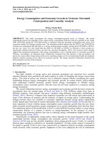
Figure 1. Line trends of tax revenue, government expenditure, and GDP per capita for
the whole sample in 2000–2015

Figure 2. Line trends of tax revenue, government expenditure, and GDP per capita

for 44 developing countries in 2000–2015



Nguyen Phuong Lien & Su Dinh Thanh / Journal of Economic Development 24(3), 04-26

23



Figure 3. Line trends of tax revenue, government expenditure, GDP per capita for 38
developed countries in 2000–2015
Source: Authors’ compilation using the data collected from IMF and WB

Appendix B
Table B

List of studied countries
Developed countries
Ord.

Country

Region(s)

Income group

1

Australia

East Asia and Pacific

High income

2

Austria

Europe and Central Asia

High income

3

Belgium

Europe and Central Asia

High income

4

Canada

North America

High income

5

Chile

Latin America and Caribbean

High income

6

Croatia

Europe and Central Asia

High income

7

Cyprus

Europe and Central Asia

High income

8

Czech Republic

Europe and Central Asia

High income

9

Denmark

Europe and Central Asia

High income

10

Estonia

Europe and Central Asia

High income



24

Nguyen Phuong Lien & Su Dinh Thanh / Journal of Economic Development 24(3), 04-26



11

Finland

Europe and Central Asia

High income

12

France

Europe and Central Asia

High income

13

Germany

Europe and Central Asia

High income

14

Greece

Europe and Central Asia

High income

15

Hungary

Europe and Central Asia

High income

16

Ireland

Europe and Central Asia

High income

17

Italy

Europe and Central Asia

High income

18

Japan

East Asia and Pacific

High income

19

Korea

East Asia and Pacific

High income

20

Latvia

Europe and Central Asia

High income

21

Lithuania

Europe and Central Asia

High income

22

Malta

Middle East and North Africa

High income

23

Netherlands

Europe and Central Asia

High income

24

New Zealand

East Asia and Pacific

High income

25

Norway

Europe and Central Asia

High income

26

Poland

Europe and Central Asia

High income

27

Portugal

Europe and Central Asia

High income

28

Seychelles

Sub-Saharan Africa

High income

29

Singapore

East Asia and Pacific

High income

30

Slovak Republic

Europe and Central Asia

High income

31

Slovenia

Europe and Central Asia

High income

32

Spain

Europe and Central Asia

High income

33

Sweden

Europe and Central Asia

High income

34

Switzerland

Europe and Central Asia

High income

35

Trinidad and Tobago

Latin America and Caribbean

High income

36

United Kingdom

Europe and Central Asia

High income

37

United States

North America

High income

38

Uruguay

Latin America and Caribbean

High income

Europe and Central Asia

Lower middle income

Developing countries
1

Armenia



Nguyen Phuong Lien & Su Dinh Thanh / Journal of Economic Development 24(3), 04-26


2

Bangladesh

South Asia

Lower middle income

3

Belarus

Europe and Central Asia

Upper middle income

4

Belize

Latin America and Caribbean

Upper middle income

5

Benin

Sub-Saharan Africa

Low income

6

Bolivia

Latin America and Caribbean

Lower middle income

7

Brazil

Latin America and Caribbean

Upper middle income

8

Bulgaria

Europe and Central Asia

Upper middle income

9

Cambodia

East Asia and Pacific

Lower middle income

10

Colombia

Latin America and Caribbean

Upper middle income

11

Congo, Rep.

Sub-Saharan Africa

Lower middle income

12

Cote d'Ivoire

Sub-Saharan Africa

Lower middle income

13

Egypt

Middle East and North Africa

Lower middle income

14

El Salvador

Latin America and Caribbean

Lower middle income

15

Ethiopia

Sub-Saharan Africa

Low income

16

Georgia

Europe and Central Asia

Upper middle income

17

Ghana

Sub-Saharan Africa

Lower middle income

18

Guatemala

Latin America and Caribbean

Lower middle income

19

India

South Asia

Lower middle income

20

Indonesia

East Asia and Pacific

Lower middle income

21

Islamic Republic of Iran

Middle East and North Africa

Upper middle income

22

Jamaica

Latin America and Caribbean

Upper middle income

23

Kenya

Sub-Saharan Africa

Lower middle income

24

Kyrgyz Republic

Europe and Central Asia

Lower middle income

25

Madagascar

Sub-Saharan Africa

Low income

26

Malaysia

East Asia and Pacific

Upper middle income

27

Mali

Sub-Saharan Africa

Low income

28

Mauritius

Sub-Saharan Africa

Upper middle income

29

Moldova

Europe and Central Asia

Lower middle income

30

Mongolia

East Asia and Pacific

Lower middle income

31

Namibia

Sub-Saharan Africa

Upper middle income

25



26

Nguyen Phuong Lien & Su Dinh Thanh / Journal of Economic Development 24(3), 04-26



32

Nepal

South Asia

Low income

33

Pakistan

South Asia

Lower middle income

34

Peru

Latin America and Caribbean

Upper middle income

35

Philippines

East Asia and Pacific

Lower middle income

36

Romania

Europe and Central Asia

Upper middle income

37

Russia

Europe and Central Asia

Upper middle income

38

South Africa

Sub-Saharan Africa

Upper middle income

39

Thailand

East Asia and Pacific

Upper middle income

40

Togo

Sub-Saharan Africa

Low income

41

Tunisia

Middle East and North Africa

Lower middle income

42

Uganda

Sub-Saharan Africa

Low income

43

Ukraine

Europe and Central Asia

Lower middle income

44

Vietnam

East Asia and Pacific

Lower middle income

Source: The World Bank