Phát triển hệ thống lưu kho tự động
Bạn đang xem bản rút gọn của tài liệu. Xem và tải ngay bản đầy đủ của tài liệu tại đây (685.6 KB, 18 trang )
TẠP CHÍ PHÁT TRIỂN KH&CN, TẬP 13, SỐ K4 - 2010
DEVELOPMENT OF AN AUTOMATED STORAGE/RETRIEVAL SYSTEM
Chung Tan Lam(1), Nguyen Tuong Long(2), Phan Hoang Phung(2), Le Hoai Quoc(3)
(1) National Key Lab of Digital Control and System Engineering (DCSELAB), VNU-HCM
(2) University Of Technology, VNU–HCM
(3) HoChiMinh City Department of Science and Technology
(Manuscript Received on July 09th, 2009, Manuscript Revised December 29th, 2009)
ABSTRACT: This paper shows the mathematical model of an automated storage/retrieval system
(AS/RS) based on innitial condition. We iditificate oscillation modes and kinematics displacement of
system on the basis model results. With the use of the present model, the automated warehouse cranes
system can be design more efficiently. Also, a AS/RS model with the control system are implemented to
show the effectiveness of the solution. This research is part of R/D research project of HCMC
Department of Science and Technology to meet the demand of the manufacturing of automated
warehouse in VIKYNO corporation, in particular, and in VietNam corporations, in general.
Keywords: automated storage/retrieval system , AS/RS model
safety condition, saving investerment costs,
1. INTRODUCTION
managing professionally and efficiently. This
An AS/RS is a robotic material handling
system has been used to supervise and control
system (MHS) that can pick and deliver
for automated delivery and picking [1], [2], [3].
material in a direct - access fashion. The
In this paper, several design hypothesis is
selection of a material handling system for a
given to propose a mathematical model and
given manufacturing system is often an
emulate to iditificate oscillation modes and
important task of mass production in industry.
kinematic displacement of system based on
One must carefully define the manufacturing
innitial conditions of force of load. As a results,
environment, including nature of the product,
we decrease error and testing effort before
manufacturing process, production volume,
manufacturing [4], [5]. No existing AS/RS met
operation types, duration of work time, work
all the requirements. Instead of purchasing an
station characteristics, and working conditions
existing AS/RS, we chose to design a system
in the manufacturing facility.
for our need of study period and present
Hence, manufacturers have to consider
several
specifications:
high
throughput
manufacturing in VietNam.
This works was implemented at Robotics
capacity, high IN/OUT rate, hight reliability
Division,
and better control of inventory, improved
Control and System Engineering (DCSELAB).
National Laboratory of Digital
Trang 25
Science & Technology Development, Vol 13, No.K4- 2010
Structural deformation is not depend on bar
2. MODELLING OF AS/RS
An AS/RS is a robot that composed of (1)
a carriage that moves along a linear track (xaxis), (2) one/two mast placed on the carriage,
axial force. Assume that the mass of each part
in AS/RS is given as m1, m2 , m3, and mL is
lifting mass.
(3) a table that moves up and down along the
When operation, there are two main
mast (y-axis) and (4) a shuttle-picking device
motions: translating in horizontal direction with
that can extend its length in both direction is
load f1; translating in vertical direction with
put on the table. The motion of picking/placing
load f2. The innitial conditions of AS/RS are
an object by the shuttle-picking device is
lifting mass, lifting speed, lifting height,
performed horizontally on the z-axis.
moving speeds, inertia force, resistance force,
In this paper, an AS/RS is considered a
none angular deflection construction in cross
section in place where having concentrated
which can be used to establish mathematical
model of AS/RS and verify the system
behavior.
The assumed parameters of the AS/RS are
mass [4], [5], [6]. There are several assumtions
given in Table 1.
as follows:
The
weight
concentrated mass
of
construction
post
is
in floor level (Fig. 1).
x3
m3
Bar 1
Bar 2
f2
K1
x1
Fig. 1: Model of AS/RS
Trang 26
L
x2
K2
mL
m2
m1
X4
f1
TẠP CHÍ PHÁT TRIỂN KH&CN, TẬP 13, SỐ K4 - 2010
Table 1 Parameters of the AS/RS
Parameter
Value
m1
150
[kg]
m2
30
[kg]
mL
100 – 500
[kg]
m3
20
[kg]
ξ
2
[%]
L
20
[m]
E
21x106
[N/cm2]
I
2.8x10³
[cm4]
k1
352.8
[N/cm]
k2
352.8
[N/cm]
kc
6594
[N/cm]
d
20
[mm]
2.1 Mathemmatical Model
k1 =
6 EI
3
x4
,
k2 =
6 EI
( L − x4 )
3
Case 1: Horizontal moving along steel
rail with load f1 [7]
with
It is assume that (1) Structural deformation
is not depend on bar axial force; (2) The mass
x4 =
where
L
, then k1= k2
2
E:
elastic
coefficient
of
material
in each part of automated warehouse cranes is
I: second moment of area
given as m1, m2 , m3, in there, mL is lifting
k1,
mass; (3)When the system moves, there are
k2
:
stiffness
proportionality
two main motions: travelling along steel rail
underload f1 and lifting body vertical direction
Case 2: Vertical moving with load f2 [8]
underload f2.
&
m2 L &
x&
4 + k c x4 + C3 x 4 = f2
The following model for traveling can be
obtained:
mL
kc
: stiffness of cable
D
: diameter of cable
&
m13&
x&
1 + k1 ( x1 − x 2 ) + C1x 1 = f1
m23 &
x&
2 + k1 ( x2 − x 1 ) + k 2 ( x2 − x3 ) = 0
&
m3 &
x&
3 + k2 ( x3 − x 2 ) + C2 x 3 = 0
where m13 = m1+ m2 + mL + m3
where m2L = m2 +
kc =
AE
π d 2E
=
4( L − x4 )
l
2.2. Solution of motion equation
a. Travelling along steel rail underload f1
m23 = m2 + mL + m3
Trang 27
Science & Technology Development, Vol 13, No.K4- 2010
If resistance force is skipped, the motion
m13 0 0
0 m 23 0
0 0 m
3
k1 -k1
0 x1
+
-k
k
+
k
-k
1 1 2
2 x2
0
-k 2
k 2 x 3
&
x&1
&
x&2
&
x&3
&+ kx = F
or in the matrix form Mx&
superposition method [9] as the followings:
Eigen problem: kφ = M φω 2 ⇒ (k − M ω 2 )φ = 0
)
that satisfy det k − M ω 2 = 0
where φ
: vibration frequency (rad/s).
x4 =
k1
} -k1
0
⇒ b = ±1.183x10
:
2
:
ω 2 = 1.135 (rad/s)
These
φ
23
-k1
k1 + k 2
-k 2
0 φ31
2
-k 2 b φ32 = ω3
k2
φ
33
−3
T
φ2 = {0.025 −0.031 −0.033}
, φ = {0.001
3
T
−0.041 0.181}
φi
:
(3)
need to be satisfied φiT kφi = ωi 2
- φ T kφ = ω 2
2
2
2
0
φ21
2 ⇒ a = ±0.025
-k 2 a φ22 = ω2
k2
(2)
φ1 values is any
T
If a and b are positive, φi values is as follows:
Trang 28
2
φ3 = {1 −34.9 153.073}
2
from the equation
2
( k − M ωi )φi = 0 are as follows:
L
-k1
k1 + k 2
-k 2
φi
2
- φ T kφ = ω 2
3
3
3
{
The solutions
ω 3 = 18.095 (rad/s)
Eq. (3), we have
b φ31 φ32 φ33
ω2 = 1.065 (rad/s), ω3 = 4.254 (rad/s).
T
Substituting constant values in Table 1 into
k1
a {φ21 φ22 φ23} -k1
0
(1)
0
φ 2 = {1 −1.252 −1.338}
k -m ω 2 -k
0
1
1 13
2
det -k1
k1 + k 2 -m 23ω
-k 2 = 0
2
-k 2
k 2 − m3ω
0
At the position
f1
0
ω 1 = 0 (rad/s)
: n level vector
ω
=
ω1 = 0 (rad/s),
Solution of Eq. (1) can be solved by
(
equation can be written as:
TẠP CHÍ PHÁT TRIỂN KH&CN, TẬP 13, SỐ K4 - 2010
It
can
be
seen
that
the
condition
T
φ M φ = I is satisfied.
T
Ri (τ ) = φi f (t )
R2 (τ ) = 0.025 f1 (t )
If resistance force is skipped, the motion
equation will be written as the followings:
R3 (τ ) = 0.001 f1 (t )
Using integral Duhamel to find motion
2
T
&
(t ) + Ω x(t ) = φ f (t )
x&
equation [9]
and n individual equation can be written:
2
&
x&
i (t ) + ωi xi (t ) = Ri (τ )
x i (t ) =
1 t
(6)
∫ R (τ ) sin ωi (t − τ ) dτ + α i sin ωi t + β i cos ωi t
ωi 0 i
R (τ )
x&i (t ) = i
sin ωi t − α iωi cos ωi t − βiωi sin ωi t
ωi
αi and βi can be specified from initial
(7)
where : ωi = ωi 1 − ξi 2
conditions
ξi : damping ratio
T
xi t =0 = φi M °u
x&i (t)=
T
x&i t =0 = φi M °u&
Geometric inversion can be defined by
principle of superposition:
u(t)=[φ ][x(t)]=[φ1 ][x1 (t)]+[φ2 ][x 2 (t)]+....+[φn ][x n (t)]
Displacement of point is defined by
principle of superposition [9]
e-ξiωit ( ( ξiωα
i i +βiωi ) sinωi t+( ξiωβ
i i - αiωi ) cosωi t )
We find αi and βi value based on initial
condition
Displacement of point is defined by
principle of superposition (Eq. (8))
n
u i (t)= ∑ φi x i (t)
i=1
Influential
Using integral Duhamel to find motion
equation [9]:
-ξ ω (t-τ)
1 t
sinωi (t-τ)dτ +
∫ R i (τ)e i i
ωi 0
-ξ ω t
e i i αi sinωi t+βi cosωi t
(
dynamic
load
act
(8)
upon
warehouse cranes in some cases
If resistance forces are considered
x i (t)=
Ri (τ)e-ξiωit ξi2ωi2
+ωi sinωi t 2
2 2
ωi +ξi ωi ωi
The acting force is a constant and system
has influential resistance force
It is assumed that f1 = Wt = 423.6 (N)
From Eq. (4) and Eq. (5), we have
)
R2 (τ ) = 0.025 f1 = 0.025 * 423.6 = 10.59 (N)
(9)
R3 (τ ) = 0.001 f1 = 0.001* 423.6 = 0.42 (N)
From Eq. (10)
Trang 29
Science & Technology Development, Vol 13, No.K4- 2010
2
2
Substituting R3 (τ ), ω3 , ξ3 into Eq. (9) and
2
2
from Eq. (9) and Eq. (11), we have α 3 = 0 ,
ω2 = ω2 1 − ξ 2 = 1.065 1 − 0.02 = 1.06 (rad/s)
ω3 = ω3 1 − ξ3 = 4.254 1 − 0.02 = 4.25 (rad/s)
Substituting the values: R2 (τ ), ω2 , ξ 2 into
β3 = 0 :
(
x 3 (t)=0.023 1-e
Eq. (9), and from initial condition:
0
T
x2 t =0 = φ2 M ° 0 = 0
0
-0.085t
( cos4.25t+0.02sin4.25t ))
with
{ω1
T
T
ω2 ω3} = {0 1.06 4.25} (rad/s)
As the results, the motion equation can be
0
T
x&2 t =0 = φ2 M ° 0 = 0
0
derived as:
From Eq. (6) and Eq. (7) with α 2 = 0 ,
β2 = 0 :
(
x 2 (t)=9.42 1-e
-0.02t
( cos1.06t+0.02sin1.06t ))
with ω3 = 4.25 :
x1 (t) 0
-0.02t
( cos1.06t+0.02sin1.06t )
x 2 (t) = 9.42 1-e
x (t)
3 0.023 1-e-0.085t ( cos4.25t+0.02sin4.25t )
(
)
(
)
(12)
With the force of load is periodic, resistance force of the system is assumed to be f1 = A cos ω t
From Eq. (4) and (5), we have
R2 (τ ) = 0.025 f1 = 0.025 A cos ωt
R3 (τ ) = 0.001 f1 = 0.001 A cos ωt
Solution x2 (t)
Substituting R2 (τ ), ω2 , ξ 2 into Eq. (9) and initial condition into Eq. (9) and Eq. (11), we have
x 2 (t ) = 22.24x10
−3
A cos ωt (1 − e
−0.02t
(cos1.06t + 0.02 sin1.06t ))
Solution x3(t)
Substituting R3 (τ ), ω3 , ξ3 into Eq. (9) and initial condition into Eq. (9) and Eq. (11), we have
-5
-0.085t
x 3 (t)=5.534x10 Acosωt(1-e
(cos4.25t-0.02sin4.25t))
Trang 30
TẠP CHÍ PHÁT TRIỂN KH&CN, TẬP 13, SỐ K4 - 2010
The motion equation under periodic load can be derived as folows:
x1 (t) 0
22.24x10⁻³ Acosωt*
(1-e-0.02t (cos1.06t+0.02sin1.06t))
x 2 (t) =
-5
5.534x10 Acosωt*
(1-e-0.085t (cos4.25t-0.02sin4.25t))
x 3 (t)
(13)
It is assumed that f = 423.6 cos 40t
1
Equation (13) becomes
x1 (t) 0
-0.02t
(cos1.06t+0.02sin1.06t))
x 2 (t) = 9.42cos40t(1-e
x (t) 0.023cos40t(1-e-0.085t (cos4.25t-0.02sin4.25t))
3
and
b. Lifting carrier in vertical direction under
load f2
defined
from
initial
condition.
when t = 0: x4 = 10 (m), x& = 1 (m/s).
4
The model of liffting carrier can be written
as
α 4 , β 4 are
(14)
(15)
&
m2 L &
x&
4 + k c x4 + C3 x 4 = f2
Substituting the values into Eq. (16), Eq. (17),
Skipping resistance force and f2 = 0, we
have x 4 (t ) = α 4 sin ω4t + β 4 cos ω4t
(16)
x&4 (t ) = α 4ω4 cos ω4t − β 4ω4 sin ω4t (17)
where ω 4 =
x i (t)=
1
ωi
kc
=
6594
m2 L
550
Oscillation system is of a harmonic motion
as
x 4 (t ) = 0.083sin11.989t + 10cos11.989t
= 11.989 (rad/s)
If resistance forces are considered, using
integral Duhamel to find the motion equation
t
∫ R (τ)e
i
-ξ i ω i (t-τ)
sinω i (t-τ)dτ+
0
e
where
we have β = 10 , α = 0.083
4
4
-ξ i ω i t
(19)
( α i sinω i t+β i cosω i t )
2
2
ωi = ωi 1 − ξi , ωi = 11.989 1 − 0.02 = 11.987 (rad/s)
α i , β i can be derived from the initial condition.
x 4 (t)=
R 4 (τ)
ω 24 +ξ 24 ω 24
-ξ 4 ω 4 t
ξ ω
(cosω 4 t+ 4 4 sinω 4 t +
1-e
ω
4
e -ξ 4 ω 4 t ( α 4 sinω 4 t+β 4 cosω 4 t )
(20)
Trang 31
Science & Technology Development, Vol 13, No.K4- 2010
R 4 (τ)e -ξ 4 ω 4 t ξ 42 ω 42
+ω 4 sinω 4 t 2
2 2
ω 4 +ξ 4 ω 4 ω 4
x&4 (t)=
(21)
e -ξ 4 ω 4 t ( ( ξ 4 ω 4 α 4 +β 4 ω 4 ) sinω 4 t+ ( ξ 4 ω 4 β 4 - α 4 ω 4 ) cosω 4 t )
when t = 0: x4 = 10 (m), x&4 = 1 (m/s).
Substituting above values into Eq. (20), we have β 4 = 10 .
(
Substituting above values into Eq. (21), we have 1= ξ 4ω4β 4 - α 4ω4
)
ξ ω β − 1 0.02 *11.989 − 1
−4
⇒ α4 = 4 4 4
=
= −63.4x10
ω4
11.987
Substituting α 4 , β 4 , ω4 , ω4 into Eq. (20), we have
x 4 (t)=
R 4 (τ)
1-e-0.24t (cos11.987t+0.02sin11.987t +
143.75
(
e
-0.24t
)
( -64.3x10
-4
sin11.987t+10cos11.987t
(22)
)
With the force of load is a costant, the resistance force is assumed to be f2 = Smax = 1736.76 N
Substituting R i (τ) = f2 = 1736.76(N) into Eq. (22):
(
( -64.3x10
)
sin11.987t+10cos11.987t )
x 4 (t)=12.08 1-e-0.24t (cos11.987t+0.02sin11.987t +
e
-0.24t
-4
(23)
Or
The force of load is periodic, the resistance force of the system is assumed to be
f2 = 1736.76 cos 40t
Substituting R i (τ) = f2 = 1736.76 cos 40t into Eq. (22)
x 4 (t)=
1736.76 cos 40t
1-e-0.24t (cos11.987t+0.02sin11.987t +
143.75
e
-0.24t
(
( -64.3x10
-4
)
sin11.987t+10cos11.987t )
(
Or x (t)=12.08cos40t 1-e-0.24t ( 0.172cos11.987t+0.02sin11.987t )
4
2.3 Simulation Results
a. The carrier travelling along rail under
load f1
Trang 32
)
(24)
From the motion equation, the system can
be simulated to describe the oscillation and
displacement of the robot on time and use Eq.
(10) to define displacement of point [10].
TẠP CHÍ PHÁT TRIỂN KH&CN, TẬP 13, SỐ K4 - 2010
The force of load is constant, the resistance
From Eq. (12), the system motion is as
force is assumed to be f1 = 423.6 (N)
follows:
x1 (t) 0
-0.02t
( cos1.06t+0.02sin1.06t )
x 2 (t) = 9.42 1-e
x (t)
-0.085t
3 0.023 1-e
( cos4.25t+0.02sin4.25t )
(
)
(
)
x1(t) = 0, the plot x2(t) and x3(t) is shown in Fig. 2.
Fig. 2. System oscillation under constant with ω = 1.06 (rad/s)
Fig. 3. System oscillation under constant load with ω = 4.25 (rad/s)
Trang 33
Science & Technology Development, Vol 13, No.K4- 2010
The point’s displacement is defined by the principle of superposition.
From Eq. (8), we have
u 1 (t)
u
(t)
2
=
u
(t)
3
(
)
0 .2 4 1 -e -0 .0 2 t ( co s1 .0 6 t+ 0 .0 2 sin 1 .0 6 t ) +
0 .2 3 x 1 0 -4 1 -e -0 .0 8 5 t ( co s4 .2 5 t+ 0 .0 2 sin 4 .2 5 t )
-0 .2 9 1 -e -0 .0 2 t ( co s1 .0 6 t+ 0 .0 2 sin 1 .0 6 t )
-4
-0 .0 8 5 t
( co s4 .2 5 t+ 0 .0 2 sin 4 .2 5 t )
9 .4 3 x 1 0 1 -e
-0 .0 2 t
( co s1 .0 6 t+ 0 .0 2 sin 1 .0 6 t ) +
-0 .3 1 -e
-4
4 1 .6 3 x 1 0 1 -e -0 .0 8 5 t ( co s4 .2 5 t+ 0 .0 2 sin 4 .2 5 t )
(
)
(
)
(
)
(
)
(
)
The point’s displacements are given in Table 2.
Table 2. The displacement of points
Time
Displace
Displace
Displace
t (s)
-ment u1 (m)
-ment u2 (m)
-ment u3 (m)
0.02
x10
0.04
-5
0.08
-5
-2.602
-4
x10
-4
-4.5204
x10-5
-1.952
x10-4
4.6777
-5.956
-4.505
x10-4
x10-4
x10-4
8.3882
-0.0011
-8.112
x10
0.1
x10
2.0415
x10
0.06
-6.1618
4.8178
-4
x10-4
0.0013
-0.0017
-0.0013
Table 3. Point Displacement
Trang 34
Time
Displace
Displace
Displace
t (s)
-ment u1 (m)
-ment u2 (m)
-ment u3 (m)
0.02
3.3624 x10⁻⁵
-4.3007 x10⁻⁵
-3.2709 x10⁻⁵
0.04
-5.971 x10⁻⁶
7.6123 x10⁻⁶
5.9202 x10⁻⁶
0.06
-3.455 x10⁻⁴
4.3995 x10⁻⁴
3.4483 x10⁻⁴
0.08
-8.387 x10⁻⁴
0.0011
8.4055 x10⁻⁴
0.1
-8.622 x10⁻⁴
0.0011
8.6695 x10⁻⁴
(25)
TẠP CHÍ PHÁT TRIỂN KH&CN, TẬP 13, SỐ K4 - 2010
With the force of load is periodic, resistance force of the system is assumed to be
f1 = 423.6 cos 40t
From Eq. (18), we have
x1 (t) 0
-0.02t
(cos1.06t+0.02sin1.06t))
x 2 (t) = 9.42cos40t(1-e
x (t) 0.023cos40t(1-e-0.085t (cos4.25t-0.02sin4.25t))
3
The oscillation plot of x2(t) and x3(t) are described in Fig. 4 and Fig. 5.
Fig. 4. System oscillation under periodic load with ω = 1.06 (rad/s)
Trang 35
Science & Technology Development, Vol 13, No.K4- 2010
Fig. 5. System oscillation under periodic load with ω = 4.25 (rad/s)
The point’s displacement is defined by principle of superposition.
From Eq. (8), we have
(
)
u 1 (t)
-0 .0 2 t
( co s1 .0 6 t+ 0 .0 2 sin 1 .0 6 t ) +
0 .2 4 co s4 0 t 1 -e
-4
-0 .0 8 5 t
( co s4 .2 5 t+ 0 .0 2 sin 4 .2 5 t )
0 .2 3 x 1 0 co s4 0 t 1 -e
u (t)
-0 .0 2 t
( co s1 .0 6 t+ 0 .0 2 sin 1 .0 6 t ) 2 -0 .2 9 co s4 0 t 1 -e
=
9 .7 4 x 1 0 -4 co s4 0 t 1 -e -0 .0 8 5 t ( co s4 .2 5 t+ 0 .0 2 sin 4 .2 5 t )
u 3 (t) -0 .3 1 co s4 0 t 1 -e -0 .0 2 t ( co s1 .0 6 t+ 0 .0 2 sin 1 .0 6 t ) +
4 2 .3 6 x 1 0 -4 co s4 0 t 1 -e -0 .0 8 5 t ( co s4 .2 5 t+ 0 .0 2 sin 4 .2 5 t )
(
(
(
)
(
(
)
)
)
)
(26)
The point displacement are given in Table 3.
b. Lifting the table in vertical direction under load f2
Resistance force is skipped and f2 = 0. From Eq. (18), the oscillation system is of harmonic motion:
x 4 (t ) = 0.083sin11.989t + 10 cos11.989t
Trang 36
TẠP CHÍ PHÁT TRIỂN KH&CN, TẬP 13, SỐ K4 - 2010
Fig. 6. Harmonic motion of system with ω = 11.989 (rad/s)
Fig. 7. System oscillation under constant load with ω = 11.978 (rad/s)
With the force of load is costant, the
resistance force is assumed to be f2 = Smax =
1736.76 N.
From
Eq.
(
-0.24t
x 4 (t)=12.08 1-e
(23),
we
With the force of load is periodic,
resistance force of the system is assumed to be
f2 = 1736.76 cos 40t
have
( 0.172cos11.987t+0.02sin11.987t ) )
Trang 37
Science & Technology Development, Vol 13, No.K4- 2010
(
From Eq. (24), we have x 4 (t)=12.08cos40t 1-e
-0.24t
( 0.172cos11.987t+0.02sin11.987t ))
Fig. 8. System oscillation under periodic load with ω = 11.987 (rad/s)
From the above plots, it can be realized
There are three computers are used to
that if we change the vibration frequency or
implement the control logic throughout the
load, the system oscillation and displacement
factory: host computer, client computer, and
will
vibration
station computer. The host computer’s function
frequency is depends on lifting body mass,
is managing the database of the system, the
lifting height, stiffness proportionality…Hence,
client computer’s function is handling in/out
if we change initial condition design, we will
operations, and the station computer’s function
iditificate oscillation modes and kinematic
is
displacement of system.
AS/RSsystem.
be
change.
Alternatively,
monitoring
and
The
controlling
control
the
system
architechture is designed to meet the demand of
3. CONTROL SYSTEM DEVELOPMENT
Trang 38
a AS/RS is shown in Fig. 9.
TẠP CHÍ PHÁT TRIỂN KH&CN, TẬP 13, SỐ K4 - 2010
Client computer with
Shopfloor Management software
Host computer with
Warehouse Management Software
LAN Network
Station Computer n
with SCADA software
Station Computer
with SCADA software
...
AS/RS
Line 1
AS/RS
Line n
Fig. 9. System control architecture for AS/RS
Fig. 10. Warehouse Management software Interface
In other words, the control system is
composed of two control levels: management
control
and
machine
control.
The
communication between them is via LAN
network. As for management control, a server
host computer is installed with Warehouse
Management software which connect to the
warehouse database using Microsoft SQL
Server framework. The server host can perform
tasks, such as supplier management, customer
management, items management, warehouse
structure management. A barcode system is
used for the item’s identification in warehouse.
The interface of Warehouse Management
software is shown in Fig. 10.
As for the machine control, a PAC
5010KW with SCADA system is implemented
to control the motion of robot for in/out
operations as shown in Fig. 11, and the control
panel on AS/RS, Fig. 12. The design has
allocated for VIKYNO company’s warehouse
as shown in Fig. 13.
Trang 39
Science & Technology Development, Vol 13, No.K4- 2010
Fig. 11. SCADA Interface and PAC 5510KW
implemented on the AS/RS model
Fig. 13. The allocation warehouse of VIKYNO for
Fig. 12. Control panel of AS/RS model
4. CONCLUSION
AS/RS implementation.
calculate program was established to verify the
behavior of the system and the system
In this paper, mathematical model of the
AS/RS is established with several oscillation
modes and the kinematic displacement of the
system are found respectively. The generalized
Trang 40
identification process. Finally, the development
of this system have been done, but the
experimental data yet to finish at this time of
this writing. It is our works in the future.
TẠP CHÍ PHÁT TRIỂN KH&CN, TẬP 13, SỐ K4 - 2010
PHÁT TRIỂN HỆ THỐNG LƯU KHO TỰ ĐỘNG
Chung Tấn Lâm(1), Nguyễn Tường Long(2), Phan Hoàng Phụng(2), Lê Hoài Quốc(3)
(1) PTN Trọng điểm Quốc gia Điều khiển số & Kỹ thuật hệ thống (DCSELAB), ĐHQG-HCM
(2) Trường Đại học Bách Khoa, ĐHQG-HCM
(3) Sở Khoa học Công nghệ Tp.HCM
TÓM TẮT: Bài báo này trình bày mô hình toán học của hệ thống lưu kho tự động (Automated
Storage/Retrieval System - AS/RS). Các chế độ giao động và chuyển vị của hệ thống được khảo sát dựa
trên mô hình cơ sở trên. Với mô hình này, việc thiết kế hệ thống robot đưa vào lấy ra sẽ hiệu quả hơn
trước khi chế tạo. Ngoài ra, một mô hình hệ thống kho hàng tự động cùng với hệ thống điều khiển đầy
đủ được thiết kế và cài đặt để thấy được sự hiểu quả của giải pháp đưa ra. Nghiên cứu này là một phần
dự án nghiên cứu chế tạo thử nghiệm của Sở khoa học Công nghệ để đáp ứng yêu cầu sản xuất kho
hàng tự động cho công ty VIKYNO nói riêng, và đáp ứng nhu cầu của các công ty Việt nam nói chung.
Từ khóa: AS/RS, Automated storage/retrieval system.
[5]. Sangdeok Park1 and Youngil Youm2,
REFERENCE
Motion Analysis of a Translating Flexible
[1]. Ashayeri, J. and Gelders, L. F, Warehouse
design optimization, European Journal of
Operational Research, 21: 285-294, 1985.
[2]. Jingxiang Gu, The forward reserve
warehouse
sizing
problem,
PhD.
Industrial
and
and
Thesis,
System
dimensioning
School
of
Engineering,
Georgia Institute of Technology, 2005.
[3]. David E. Mulcahy, Materials Handling
Handbook,
Published by McGraw-Hill
Professional, 1999.
[4]. Kim
H-S
(Korea
Maritime
Univ.),
Ishikawa H (Kongo Corp.), Kawaji S
(Kumamoto
Univ.),
Control
High
for
Stacker
Rack
Crane
Warehouse
Systems, Vol. 2000; No. Pt.1, 2000.
Beam
Carrying
a
Moving
Mass,
International Journal Korean Society of
Precision Engineering, Vol. 2, No. 4,
November, 2001.
[6]. GS. TSKH. Võ Như Cầu, Tính toán kết
cấu theo phương pháp động lực học, Nhà
xuất bản xây dựng Hà Nội, 2006.
[7]. Ing.J.Verschoof, Crane Design, Practice,
and
Maintenance,
Professional
Engineering Publishing Limited London
and Bury StEdmunds, UK, 2002.
[8]. Huỳnh Văn Hoàng, Trần Thị Hồng,
Nguyễn Hồng Ngân, Nguyễn Danh Sơn,
Lê Hồng Sơn, Nguyễn Xuân Hiệp, Kỹ
thuật nâng chuyển, Nhà xuất bản Đại Học
Quốc Gia TPHCM, 2004.
Trang 41
Science & Technology Development, Vol 13, No.K4- 2010
[9]. Nguyễn Tuấn Kiệt, Động lực học kết cấu
cơ khí, Nhà xuất bản Đại học quốc gia Tp.
Hồ Chí Minh, 2002.
[10]. Nguyễn Hoài Sơn, Vũ Như Phan Thiện,
Đỗ Thanh Việt, Phương pháp phần tử
Trang 42
hữu hạn với Matlab, Nhà xuất bản Đại
học quốc gia Tp. Hồ Chí Minh, 2001.
![PHÁT TRIỂN HỆ THỐNG TÁI SINH TỪ MÔ SẸO PHỤC VỤ CHỌN DÒNG CHỊU HẠN Ở CÂY ĐẬU TƯƠNG [GLYCINE MAX(L.) MERRILL]](https://media.store123doc.com/images/document/13/ri/vx/medium_vxb1366606649.jpg)