On a programme for the balancing calculation of flexible rotors with the influence coefficient method
Bạn đang xem bản rút gọn của tài liệu. Xem và tải ngay bản đầy đủ của tài liệu tại đây (1.12 MB, 13 trang )
Vietnam Journal of Mechanics, NCST of Vietnam Vol. 22, 2000, No 4 (235 - 247)
ON A PROGRAMME FOR THE BALANCING
CALCULATION OF FLEXIBLE ROTORS WITH
THE INFLUENCE COEFFICIENT METHOD
NGUYEN VAN KHANG - TRAN VAN LUONG
Hanoi University of Technology
ABSTRACT. This paper presents the influence coefficient method of determining the
locations of unbalances on a flexible rotor system and the correction weights. A computer
software for calculating the at-the-site balancing of a flexible rotor sys.tern was created
using c++ language at the Hanoi University of Technology. This software can be used
by balancing flexible rotors in Vietnam.
1. Introduction
The well-known methods of the at-the-site balancing of flexible rotors (the
method of three time starting the trial weights, the vector triangle, the sensitivity)
were successfully used to balance separate flexible rotors at the site. However, the
efficiency of these balancing methods depends a lot on the correctness of the analysis of the vibration modes of separate rotors. Nowadays, rotors are manufactured
longer and longer, many rotors are connected with each other. After manufacture,
rotors are separately balanced before leaving the production workshop, but by
connecting many rotors together, the separate balance status disappears due to
mutual interaction of the residual unbalance remaining in each rotor which causes changes in the vibration of the entire system. The methods of separate rotor
balancing may reduce vibration of the balanced rotor, but may increase vibration
in many points in the other rotors of the system. In order to work safely, the
vibration rate in all points of the rotor system, in all regimes, must lie within the
permitted standards. Therefore the entire system of rotors must be balanced.
In this paper, the author present the influence coefficient method for balancing flexible rotors [1, 2, 3]. This method is dependent on the basic principle that
the influence coefficient matrix is square. In actual balancing, however, the influence coefficient matrix is not necessarily square but is often a non-square matrix.
The least-squares balancing method is a method in which correction weights are
calculated under the condition of minimizing the sum of the squares of residual
235
vibrations. From this method the computer software for the calculation of the
at-the-site balancing of a flexible rotors system was created using c ++ language
at the Hanoi University of Technology.
2. Theoretical basis of a programme for balancing calculation
2.1. Concept of influence coefficient
Let us call Tj the vibration at the measured point j (j = 1, ·... , J, depending
on the measured point and the speed number), Tjk measurement results at y" due
to unbalance U in plane k at rotor speed 0, we obtain the following formula:
(2.1)
where ""ii.jk is the proportion coefficient. This coefficient shows the influence of
unbalance Uk on the measurement results at jth measured point and is called the
influence coefficient.
For convenience, let's have Tjk and Uk in the form of complex numbers,
therefore ""ii.jk will also be calculated in complex number.
2.2. Determination of influence coefficients with measurement of vibration
The initial unbalance vibration at the measured point j, (j = 1, ... , J) is rf vibration at
y"th measured point with trial weight Uk is r~
and we have
(2.2)
From ( 2 .1) we will have
_
O'.jk
=
Tjk
~
Uk
-M
=
Tjk -
-A
TJ·
(2.3)
Uk
Fig . 1
The unit of ""ii.jk is [m/kg ] or [mm/g]. By changing the test weights at the balancing plane k (k = 1, ... , K) we will determine the influence coefficients ""ii.jk
U = 1, ... , J), (k = 1, ... , K).
2.3. Influence coefficient matrix and determination of the correction
weights
The vibration at Jih point on the rotor due to separate unbalancing
1, ... , K) at all balancing planes according to formula (2.1) is
236
Uk
(k =
K
ri
=
K
L:rjk
L:ajkuk (j
=
k=l
= 1, ...
,J).
(2.4)
k=l
The system of algebraic equation (2.4) may be rewritten in the matrix form as
follows
[
~1]
r2
..
.
[au
0:21
-
.
(2.5)
..
an
TJ
O'.J2
If we use the following symbols
r=
[:J; [
A=
~11
0'.21
.
(2.6)
the equation (2.5) will be
r=A·U .
(2.7)
The matrix Ais a complex matrix of size J x K and is called the influence coefficient
matrix. The correction weights Uk (k = 1, . . . , K) must be calculated from the
balancing condition
-A
-A
Q
(2.8)
rj=-ri
=;.ri+ri
=.
In practice there is always residual unbalance vibration ;;;! , we have
(2.9)
Substituting (2.7) into (2.9), we obtain
(2.lOa)
or
K
rf = rf + Laikuk
(j = 1, ... ,J).
(2.lOb)
k=l
If A is a square and has det A -::/= 0 then from the equation (2.10) we may
solve U. In actual balancing, however, the influence coefficient matrix A is not
necessarily square but often a non-square matrix. We will consider the following
\
cases:
237
a} Case 1: J = k (the number of measured points is equal to the number of
the balancing planes). In this case matrix A is square. Assuming that det A f. O
and from (2.lOa) we obtain
U = -A- 1(rA - r').
(2.11)
When rf = O, we have the formula to determine the correction weights U
(2.12)
According to (2.12) we can determine the 'correction weights Uk (k = 1, ... , K)
b) Cases 2: J > K (the number of measured points is more than the number
of the balancing planes). This is the case often met in technical practice provided
that rf = 0, and from (2.lOa) we have
AU= -rA,
(2.13)
where A is non-square. We have J equations and unknown (K < J) . The problem
has many roots . We have to find out the optimal root. We will adjust the errors
and see (2.lOa) or (2.lOb) as the error equation and use the least square method
to deal with a goal that the total sum of squares of errors is minimum.
The total sum of errors is as follows:
J
J
L lr'l2 = l:r{. (r{)*,
F =
i=l
where
r{ =
i=l
+ i(rf)",
(-I)
ri * -_ ( riI) ' - i ·(riI) " .
Let's mark Uk = U~
+ iU~'
(2.14)
(rf)'
(2.15)
then (2.lOb) will be:
K
-f
-A
ri =ri
"°' -
+ L-Ct.ik (U'k + i'U")
k
i=l
K
(2.16)
(rf)* = (rf )* + L ajk(Uk - iUf:)
k=l
By substituting (2.16) into (2.14) F is a function with real variables U~ and Uf:
(k = 1, ... ,K)
(2.17)
F = F(U~ ... U~, U~' ... U~).
238
The condition for function F to reach minimum is:
BF
au'k
=
o;
BF
au" = o (k=l, ... ,K).
(2.18)
k
Thus, as conditions for seeking the correction weights Uk and Uf: that minimize
equation (2.17) under equations (2.14) and (2.16) , the following equations must
be obtained:
a-I
a(-f) *
ri
au' - ~ au' (rj) + au' rj - o, (k
BF _ "
k
J
-!] _
[ r i -f *
j=l
k
k
J
a-I
a(-f) *
aF - " [ r j - f *
rj
-!]
au" - ~ au" (rj ) + au" r j
k
k
j=l
k
- o,
-
,K) ,
(2.19a)
(k = l, ... ,K).
(2.19b)
= 1, ...
By substitut ing (2.16) into (2.19) and rearranging the results , the following equations are derived:
J
J
I: [aik(rJ) * + -aikrf] = 2 I: Re(ajkr{) = o, (k = 1, ... , K),
j =l
j =l
J
L
(2 .20)
J
[iaik(r{)* - iajkrf] = 2 L Im(ajkrJ) = o, (k = 1, ... , K).
j=l
(2.21)
j=l
The equations (2.20) may be rewritten as follows
(2.22)
or in the matrix equation as
Re
[~!1
0'.12
aiK
_.,
-·
-·
0'.21
0'.22
~{·]
aJ2
-f
r2
_.,
-!
O'.JK
a2K
-f
ri
.
=0,
(2.23)
TJ
=> Re[(A*)Trt] -:- o.
(2.24)
With similar changes to those made to equation (2.21) we have
(2.25)
'239
(A") T is the transported matrix of the complex combined matrix A*. Because A is a matrix of size J x Kth.en (A*) T .is also of size K x J. The equations
where
(2.24) and (2.25) may be rewritten as follows
(2.26)
By substituting (2.lOa) into (2.26), we have
(2.27)
Noting that (A*) T ·A is the square matrix of K degree and will not be irregular,
therefore from (2 .27) we can find the correction weights
(2.28)
3. Flow chart of the programme for balancing calculation
The calculation of a system of correction weights is equivalent to the solving of
equation (2.28) and shall be implemented with computer software written inc++
language. Fig. 2 is a fl.ow chart of the above balancing method. In this method,
the influence coefficient can be obtained by either calculation or measurement.
4. Experimental results of verification on
mod~ls
In order to verify the correctness of the algorithm and the reliability of the
computer calculation programme, the tests were made on rotor model KIT, Model
24750 Bently Nevada (USA), equipment LeCroy 9304A QUAD 200 MHz Oscilloscope {USA).
4.1. Experimental model
Rotor KIT is an experimental model for the research of flexible rotor balancing
(Fig. 3), including a motor with adjustable speeds between 0 and 10,000 rpm, a
shaft, bearings, two balancing disks with caving-off holes which are proportionally
located on such disks for mounting the correction weights. Distance between disks
and distance between bearings are also adjustable. Vibration at all points on the
shaft are measured with non-contact bridge meters.
240
IMeasurement of the initial vibration I
Y1e· s
Is the vibration
Yes
Selection of balancing speeds, planes and test weight
Vibration with presence of the test weights
Determination of the influence coefficient matrix
Computing of correction weights
l
1
Acceleration operation after adding the correction weights
No
Is the vibration
amplit ude allowable ?
Yes
\ End of balancing
J
Fig. 2. Flow chart of balancing
241
No need for
balancing
X-Y PROSE
MOIJNT AND PROS S
HOl..ES EVENL.V
SPEED AlONG
ENTRE LENGTH
iNSOARP
BEARiNO HDUSiNG
MOTOR SPEED CONTROl
Fig. 3. Model of rotor KIT for the balancing experiment
In Fig. 4 the scheme of the tests is described.
(2)
(3)
Motor
Speed
(4)
nt
========n~LJ
Phase measurement signal
measurement
Fig. 4. The principle Scheme of Tests
(0)-Signal for adjustment of the revolution, (1)-key phase, (2), (3), (4) measured points;
(I), (II) - balancing planes, (5) - Amplification of signals, (6) - Display of vibration
4.2. Experimentat results
a) Initial vibration. The rotor revolves with certain speeds and vibration is
measured at various measured points before balancing as indicated in Tab. 4.1.
Rotor
speed,
rpm
3000
2700
2400
1800
Vertical amplitudes at measured points 2A/cp, µm/degree
(2)
(3)
(4)
85.3/39.3
93/4'.l.6
242/22.8
46.9/351.5
340/83.8
547.5/64.5
878/34.5
240/44.7
89.9/172
78.13/126.1
119/67.6
13.3/264
242
b} Calculation of balancing added weights. The balancing added weigh.ts shall
be calculated according to the programe:
U1 = 2.16/18 gram/degree; U2 = 1.17 /274 gram/degree.
The balancing added weights shall be mounted on the rotor KIT:
U1 = 2/22,5 gram/degree; U2 = 1.2/270 gram/degree
Vibration at the measured points at speed of 3000 rpm, after the balancing
(Fig.Sa, b, c):
Measured object Measured point (2)
2A/cp
Measured point (3)
Measured point ( 4)
103.8/86
55.8/234
17.6/198
The balancing quality [4] for all measured points at speed of n = 3000 rpm is
K = 0. 71. The balancing has reached good results and proved the correctness of
the algorithm and the programme. The vibrations before balancing and vibrations
after balancing are shown in Fig. Sa, b and c.
5. Conclusion
The influence coefficient method allows us to optimize the system of added
balancing weights for all balancing planes at various speeds. It does not depend
on types of bearing or pivots, does not limit the number of bearings pivots or the
number of shafts in one system of shafts, or the modes of eigenvibration of each
shaft, each system of shafts. The least squares method was used to deal with
. errors in the calculation of the correction weights and the determination of the
members of the matrix of influence coefficients. We can determine the system of
added correction weights to assure the efficiency of the balancing process.
The computer software for calculating the correction weights for the at-thesite balancing of the system of flexible rotors, which has been well verified by tests
on various models now allows us to carry out the balancing of the entire system
of flexible rotors with high efficiency.
This publication is completed with the financial support of the Council for
Natural Sciences of Vietnam.
243
2
Amplitude at point (2) before balancing at n = 3000 rpm
2
Amplitude at point (2) after balancing at
n = 3000
rpm
Before balancing: 2A/cp = 85.8/39.3 µm/degree
After balancing: 2A/cp
·, -
= 17.6/198 µm/degree
--
Fig. 5a. Amplitudes at point (2) before and after balancing
244
3
--j
Amplitude at point (3 ) before balancing at n
=
3000 rpm
3
Amplitude at point (3) after balancing at
n =
3000 rpm
Before balancing: 2A /cp = 430/83.8 µm/degree
After balancing: 2A/cp = 103.8/86 µm / degree
Fig. Sb. Amplitudes at point (3) before and after balancing
245
Amplitude a t point (4) before balancing at n
=
3000 rpm
!
i
--- - "
iI
,,
L
r
J
f\..
.~
'
l
r
'\
.\.
l
\
~\
I
I.
\
n
J
.
\ \ \ \ \ : \
\J \}• \J \J. t. \J. \1. ' ' t \) \i
"
\
I
~
i
I
Amplitude at point (4) after balancing at
n = 3000
rpm
2A / 2A j F ig. Sc . Amplitudes at point (4) before and after balancing
Before balancing:
After balancing:
246
-
REFERENCES
1.
Tran Van Luong. Investigation of vibration and balancing at the site of flexible
rotors system in power station. Doctor thesis (draft) Hanoi University of
Technology, 2000.
2.
Fujisawa F., Shiohata K. , Sato K ., Imai T ., Shoyama E. Experimental investigation of multi-span rotor balancing using least squares method . J. of
Mechanical Design, Vol. 102, 1980, pp. 589-596.
3.
Rao J . S. Rotor Dynamics , Wiley Eastern Limited, New Delhi 1983.
4.
Kellberger W . Elastisches Wuchten, Springer-Verlag, Berlin 1987.
Received August 3, 2000
""
.....
""
""
,
,
....
~
'
VE MQT PHAN MEM TINH TOAN CAN BANG CU A
,..
H~
....
ROTO
DANH51BlNGPHUONGPHAPHts6ANHHU6NG
Trong cong trlnh nay xet vi~c Stf dvng phrrcmg phap h~ so anh hrr&ng ket
h<;YP v&i phrrOTig phap blnh phmmg toi thi~u d~ xac d!nh cac v! trf mat can b~ng
va tinh toan gia tr9ng can b~ng cho h~ roto dan hoi. MC}t phan mem tinh toan
can bKng t~i ch6 cho h~ roto dan hoi da dm:_yc xay dl!ng & D~i hNC}i. Tir d6 m& ra m9t kha nang m&i cho vi~c giai quyet cac bai toan can b~ng
h~ roto phrrc t~p 6' cac nha may di~n cung nhll' 6' cac Xl nghi~p CO Stf dvng CaC h~
roto.
247