A fast fuzzy finite element approach for laterally loaded pile in layered soils
Bạn đang xem bản rút gọn của tài liệu. Xem và tải ngay bản đầy đủ của tài liệu tại đây (539.73 KB, 9 trang )
Journal of Science and Technology in Civil Engineering NUCE 2018. 12 (3): 1–9
A FAST FUZZY FINITE ELEMENT APPROACH
FOR LATERALLY LOADED PILE IN LAYERED SOILS
Pham Hoang Anha,∗
a
Faculty of Building and Industrial Construction, National University of Civil Engineering,
55 Giai Phong road, Hai Ba Trung district, Hanoi, Vietnam
Article history:
Received 05 October 2017, Revised 05 March 2018, Accepted 27 April 2018
Abstract
A fuzzy finite element approach for static analysis of laterally loaded pile in multi-layer soil with uncertain
properties is presented. The finite element (FE) formulation is established using a beam-on-two-parameter
foundation model. Based on the developed FE model, uncertainty propagation of the soil parameters to the
pile response is evaluated by mean of the α-cut strategy combined with a response surface based optimization
technique. First order Taylor’s expansion representing the pile responses is used to find the binary combinations
of the fuzzy variables that result in extreme responses at an α-level. The exact values of the extreme responses
are then determined by direct FE analysis at the found binary combinations of the fuzzy variables. The proposed
approach is shown to be accurate and computationally efficient.
Keywords: laterally-loaded pile; uncertainty; fuzzy finite element analysis; α-cut strategy; response surface
method; optimization.
c 2018 National University of Civil Engineering
1. Introduction
Piles subjected to lateral loadings can be found in many civil engineering structures such as offshore platforms, bridge piers, and high-rise buildings. For the design of pile foundations of such
structures, special attention needs to be concentrated not only on the bearing capacity but also on the
behavior (horizontal displacement, stress) of the piles under lateral loading conditions. The deterministic analysis of lateral loading behavior of piles is complicated and in general requires a numerical
solution procedure (e.g., the finite difference method, finite element method).
On the other hand, uncertainty is often present in the input data, especially in geotechnical engineering data. These uncertainties can be accounted for by using probabilistic methods, e.g., methods
proposed in [1–6]. However, very often the input data fall into the category of non-statistical uncertainty. The reason for this uncertainty is that the made observations could be best categorized with
linguistic variables (e.g., the soil may be described with linguistic variables such as “very soft,” “soft,”
or “stiff”; “loose”, “dense”, or “very dense”), or that only a limited number of samples are available
∗
Corresponding author. E-mail address: (Anh, P. H.)
1
Anh, P. H. / Journal of Science and Technology in Civil Engineering
and a particular soil properties are unknown or vary from one location to another location. These
types of uncertainties can be appropriately represented in the mathematical model as fuzziness [7].
In recent years, non-probabilistic FE methods based on fuzzy set theory have been introduced
to the analysis of uncertain structural systems. The fuzzy FE methods have been applied for both
static and dynamic analysis of various structures [8–11]. In this paper, an efficient fuzzy FE approach
is developed to analyze the response of laterally loaded pile in multi-layer soils. It is assumed that
only rough estimates of the soil parameters are available and these are modeled as fuzzy values. The
analysis of the pile-soil interaction is based on a “Beam-on-two-parameter-linear-elastic-foundation”
FE model. The fuzzy pile response is estimated by a response surface based optimization technique
using first order Taylor’s expansion of the pile response. The accuracy and computational efficiency
of the proposed approach are illustrated in a numerical example.
xxx
2. 2.1
General
fuzzy structural
analysis
Fuzzy model
of uncertainty
practical
engineering
problems,
2.1.In Fuzzy
model
of uncertainty
there are randomness and fuzziness associated with the model
parameters (e. g. material properties, geometrical dimensions, loads). These uncertainties can be modeled
randomness
andasfuzziness
theand
model
X (Xare
, Xassociated
) with X with
inAmong
form of practical
fuzzy setsengineering
[7]. Accordingproblems,
to [7] a fuzzy
set is defined
is a set
parameters (e.g. material properties, geometrical dimensions, loads). These uncertainties can be
[0,1]
X ,µthe
function. Corresponding to each element ˜x
value
X
modeled
in form isofcalled
fuzzythe
setsmembership
[7]. According
to [7] a fuzzy set is defined as X = (X,
X ) with X is
a set Xand
→ [0,membership
1] is calledlevel
the of
membership
totoeach
element
X, the
(x )µisX called
defines theCorresponding
level of x belong
the fuzzy
set Xx .∈The
x ; X (x ) function.
˜
value µX (x) is called membership level of x; µX (x) defines the level of x belonging to the fuzzy set X.
value 0 state that x is not belong to X ; the value
1 means that x is definitely belong to X ; the value ˜in
˜
The value 0 states that x does not belong to X; the value 1 means that x definitely belongs to X; the
X is uncertain.
interval
0 to 1 shows
the level
x belonging
value
in interval
0 to 1that
shows
thatofthe
level of xtobelonging
to X˜ is uncertain.
The α-cut, X of the fuzzy set X˜ is a set of elements xX∈ X
with the membership level
α:
(x )µX (x) ≥
The α-cut, X αof the fuzzy set X is a set of elements x
with the membership level
:
X
X{
∈X
1]
α x= {xX
: : Xµ(Xx(x)
) ≥ α},
}, α ∈ [0,[0,1]
X
Fig.1 1illustrates
illustrates
membership
function
of a triangular
Fig.
the the
membership
function
and an and
α-cutan
of α-cut
a triangular
fuzzy set.
(1)
(1)
fuzzy set.
μX (x)
Xα
α
xα,min
x, X
xα,max
Figure
andthe
theα-cut
α-cutofofa afuzzy
fuzzy
Figure1.1.Membership
Membership function
function and
setset
2.2 The α-level optimization
2.2.Consider
The α-level
optimization
a model output y
given by
y
f (x1, x 2,..., xn ) with x i being n
fuzzy input variables,
output
by y = f (x1 , xbe
. . , xfunction
being n model,
fuzzy input
variables,
2 , . any
n ) withorxinumerical
xConsider
Xi : a model
[0,1]y. given
The function f ( ) can
e.g. the finite
i
Xi (x )
xi ∈ Xi : µXi (x) →
[0, 1]. The function f (·) can be any function or numerical model, e.g. the finite
element model. Through the mapping function f ( ) , the output y is also a fuzzy quantity represented by
2
its output fuzzy setY
{y
Y :
Y (y )
[0,1]} . A practical mean to determine the membership
function of y , Y (y ) , is the α-cut strategy [8]. Here, the fuzzy input variables are discretized into
levels,
k ,(k
= 1,2,...,m ) . Corresponding to each level
k
m
, we have crisp sets of values of inputs,
Anh, P. H. / Journal of Science and Technology in Civil Engineering
element model. Through the mapping function f (·), the output y is also a fuzzy quantity represented
by its output fuzzy set Y˜ = {y ∈ Y : µY (y) → [0, 1]}. A practical mean to determine the membership
function of y, µY (y), is the α-cut strategy [8]. Here, the fuzzy input variables are discretized into
m levels, αk , (k = 1, 2, . . . , m). Corresponding to each level αk , we have crisp sets of values of
˜ is then
inputs, Xi,αk ⊂ Xi . The output interval of y corresponding to level αk (the αk -cut Yαk of Y)
determined by interval analysis of the input sets Xi,αk through the mapping model f (·). Thus, a
discrete approximation of the membership function of the output can be obtained by repeating the
interval analysis on a finite number of αk -levels. Fig. 2 illustrates the fuzzy analysis using the α-cut
xxx
strategy for a function of two input variables.
αk
Interval analysis
of level α
x1
αk
y
αk
x2
Figure 2. Illustration of fuzzy analysis by α-cut strategy
Figure 2. Illustration of fuzzy analysis by α-cut strategy
The smallest and largest values (the extreme values) of the α-cut Y define two points of the membership
k
The smallest and largest values (the extreme values) of the α-cut Yαk define two points of the
function of the fuzzy output, Y . The exact extreme values of the α-cut Y are often determined by
˜ The exact extreme valuesk of the α-cut Yαk are often
membership function of the fuzzy output, Y.
solving two optimization problems, which referred as the α-level optimization [12]:
determined by solving two optimization problems, which are referred as the α-level optimization [12]:
y
y
min
,min
f (x1, x 2 ,..., x n )
Xi ,
ykαk ,min =xi min
k ( f (x1 , x2 , . . . , xn ))
xi ∈Xi,αk
m ax
k ,m ax
f (x1, x 2 ,..., x n )
(2)
(2)
Xi ,
k ( f (x , x , . . . , x ))
yαk ,max = ximax
1 2
n
xi ∈Xi,αk
The solution for the optimization problems of Eq. 20 can be numerical demanding. In order to reduce the
computational burden, researchers have focused on efficient procedures to reduce the number of function
The
solution
for the optimization
problems
Eq. (2) can be numerical demanding. In order
evaluations
in performing
these optimization
problemsof[8,10,11].
to reduce the computational burden, researchers have focused on efficient procedures to reduce the
This paper introduces a fast solution for the above optimization problems based on a response surface
number
of function
evaluations
in performing
optimization
problems
[8, 10,
method,
which is applicable
for the
fuzzy analysisthese
of laterally
loaded piles
with uncertain
soil 11].
parameters. The
methodology
is presentedainfast
the followings.
This
paper introduces
solution for the above optimization problems based on a response
3. Fuzzy
finite
element
analysis of laterally
loadedanalysis
pile
surface
method,
which
is applicable
for the fuzzy
of laterally loaded piles with uncertain soil
parameters. The methodology is presented in the followings.
3.1 Model of analysis
Consider
a vertical
pile embed
in aof
soillaterally
deposit containing
n layers, with the thickness of layer i
3. Fuzzy
finite
element
analysis
loaded pile
3.1.
given by Hi
(Fig. 1(a)). The top of the pile is at the ground surface and the bottom end of the pile is considered embedded
in the nof
-thanalysis
layer. Each soil layer is assumed to behave as a linear, elastic material with the compressive
Model
resistance parameter ki and shear resistance parameter ti . The pile is subjected to a lateral force F0 and a
Consider
a vertical pile embed in a soil deposit containing n layers, with the thickness of layer i
moment M 0 at the pile top. The pile behaves as an Euler–Bernoulli (EB) beam with length Lp and a constant
given by Hi (Fig. 3(a)). The top of the pile is on the ground surface and the bottom end of the pile
flexural rigidity EI . The governing differential equation for pile deflection wi within any layer i is given in [13]:
is considered
embedded in the n-th layer. Each soil layer is assumed to behave as a linear, elastic
material with the compressive resistance
parameter ki 2and shear resistance parameter ti . The pile
4
EI
d wi
dz
4
kiwi
2ti
3
d wi
dz 2
0
(3)
The equation (3) is exactly the same as the equation for the “Beam-on-two-parameter-linear-elasticfoundation” model introduced by Vlasov and Leont’ev [14]. The use of linear elastic analysis in the laterally
loaded pile problem, especially in the prediction of deformations at working stress levels, has become a
widely accepted model in geotechnical engineering. Also in the real problem where nonlinear stress-strain
relationships for the soil must be used, linear elastic solution provides the framework for the analysis, in which
Anh, P. H. / Journal of Science and Technology in Civil Engineering
is subjected to a lateral force F0 and a moment M0 at the pile top. The pile behaves as an Euler–
Bernoulli (EB) beam with length L p and a constant flexural rigidity EI. The governing differential
equation for pile deflection wi within any layer i is given in [13]:
EI
d4 wi
d 2 wi
+
k
w
−
2t
=0
i
i
i
dz4
dz2
(3)
Eq. (3) is exactly the same as the equation for the “Beam-on-two-parameter-linear-elasticfoundation” model introduced by Vlasov and Leont’ev [14]. The use of linear elastic analysis in
the laterally loaded pile problem, especially in the prediction of deformations at working stress levels, has become a widely accepted model in geotechnical engineering. Also in the real problem
where nonlinear stress-strain relationships for the soil must be used, linear elastic solution provides
the framework for the analysis, in which the elastic properties of the soil will be changed
xxxwith the
changing deformation of the soil mass (e.g., the “p–y” method [15]).
this paper, this Beam-on-linear-elastic-foundation model is the basis for the finite element formulation
of
xxx
xxx
InIn
this
paper, this Beam-on-linear-elastic-foundation model is the basis for the finite
element
the laterally loaded pile problem which will be presented in the next section.
formulation
of
the
laterally
loaded
pile
problem
which
will
be
presented
in
the
next
section.
InInthis
paper,
this
Beam-on-linear-elastic-foundation
model
is
the
basis
for
the
finite
element
formulation
of
this paper, this Beam-on-linear-elastic-foundation model is the basis for the finite element formulation of
the
problem
which
in in
thethe
next
section.
thelaterally
laterallyloaded
loadedpile
pile
which
presented
next
section.
M
0problem
F0 willwillbebepresented
MM
0 0
Layer 1
F0F0
H1
Layer
11
Layer
H1H1
Layer
22
Layer
H2H2
Layer 2
…
w
ww
ww
Beam-type element
H2
qjθ
…
Lp
LpLp
……
w
node j
……
Layer i
qjθqjθ
nodej j
node
w2, Q2
Hi
Layer
Layer
i i
HiHi
…
……
w2w
, Q2,2Q2
,M2,M
θ
θθ22,M
22 2
…
……
Layer
Layer
Layern nn
zz z
z zz
zz z
(a)
(a)
(a)
(a)
Figure 3. (a)
qjw
qjwqjw
Beam-type
Beam-type
θelement
M1
1, element
θ1,M
θ1,M
1 1
we
w1, Q1 wewe
w1w
,Q11,Q1
le
le le
(b) (b)
(b)
(b)
(c)
(c)(c)
(c)
Figure3.3.(a)(a)A A
laterally-loaded
pile
a layered
soil;
discretization;
laterally-loaded
pile
in in
asoil;
layered
(b)(b)
FEFE
discretization;
AFigure
laterally-loaded
pile in a layered
(b) soil;
FE
discretization;
(c) Beam-type
Figure 3. (a) A laterally-loaded
pile
in
a
layered
soil;
(b)
FE
discretization;
(c)
Beam-type
element
(c) Beam-type element
3.2 Finite element modeling
3.2 Finite element modeling
element
(c) Beam-type element
3.2. The
Finite
element
3.2
Finite
elementmodeling
modeling
pile is divided into m finite elements and to each j -th node of their interconnection, two degrees of
The pile is divided into m finite elements and to each j -th
node of their interconnection, two degrees of
q j each
The
pileare
divided
m deflection
finite
elements
and
each
node
of with
theirpositive
interconnection,
freedom
allowed:
–finite
the
andq to
–
thej to
rotation
ofj-th
cross
section
directionofas two
q into
The pile
isisallowed:
divided
into
elements
and
-th
node
theirsection
interconnection,
twodirection
degrees
m
freedom
are
– the
deflection
and
–
the
rotation
of of
cross
with positive
as
q jwjw
j
degrees
of
freedom
are
allowed:
q
the
deflection
and
q
the
rotation
of
cross
section
with
jw is chosen
jθ
q
in
Figure
1(b).
Element
of
EB-beam
type
for
each
pile
element
with
length
and
two
nodes,
l
freedom
are allowed:
– the deflection
and
theeach
rotation
ofelement
cross section
with positive
as
qofjw EB-beam
j –for
eand direction
in
Figure
1(b).
Element
type
is
chosen
pile
with
length
two
nodes,
l
e
positive
direction
in element
Fig. 3(b).
Elementtoofother
EB-beam
forToeach
element
one at
each end.asThe
is connected
elementstype
only is
at chosen
the nodes.
eachpile
element,
two with
one
at each
end.Element
The element
is
connected
to
other
elements
only
at the with
nodes.
To
each
element,
two at the
in
Figure
1(b).
of
EB-beam
type
is
chosen
for
each
pile
element
length
and
two
nodes,
l
length
l
and
two
nodes,
one
at
each
end.
The
element
is
connected
to
other
elements
only
e
degrees of freedom are allowed at both ends: deflection, w and rotation,
, and we ,
respectively,
degrees of freedom are allowed at both ends: deflection, w 1 1and rotation, 1 , 1and w 2 , 2 2 2respectively,
oneTo
at each
each element,
end. The element
is connected
to otherare
elements
only
atboth
the ends:
nodes. deflection,
To each element,
tworotation,
nodes.
two
degrees
of
freedom
allowed
at
w1 and
positive in the system of local axes as shown in Figure 1(c). The element nodal displacement vector
q e
positive
in
the
system
of
local
axes
as
shown
in
Figure
1(c).
The
element
nodal
displacement
vector
q
degrees
are allowed
at both
deflection,
rotation,
, 2 3(c).
respectively,
θ1 , and
w2 , θof2 freedom
respectively,
positive
in ends:
the system
of wlocal
as shown
Thee element
w 2Fig.
1 andaxes
1 , and in
and the element nodal force vector r
with respect to the system of local axes are defined:
nodal
displacement
vector
element
nodal
force
vector
with
respect
to the system of
{q}
{r}edisplacement
ewith
and
the element
nodal
force
vector
respect
to1(c).
the system
of local
axes
are defined:
e and
r the
positive
in the system
of local
axes
as
shown
in Figure
The element
nodal
vector
q e
e
local axes are defined:
T
T
(4)
w r w withT respect
,
rto the system
Q1 M
Q2 M
and the element nodalqforce
vector
of1local
axes
2T are defined:
(4)
q e e w1 1 1 1w2e 2 2 2 , T r e e Q1 M
Q2 M
T
1
2
(4)
{q}e = {w1 θ1 w2 θ2 } , {r}e = {Q1 M1 Q2 M2 }
It is noted that Q 1 and Q 2 from (4) include shear
T force in the pile section and also
T shear force in the soil.
It is noted that Q 1 and Q
shear ,forcerin
also shear force in the soil.(4)
q 2 efrom (4)
w1include
M1 Qand
4 ethe pileQ1section
1 w2 2
2 M2
The equilibrium equation of an element has the form:
The equilibrium equation of an element has the form:
It is noted that Q1 and Q 2 from (4) include kshearqforce in the
r pile section and also shear force in the soil. (5)
k eq e r e
(5)
e
e
e
The
equilibrium
has
form: the stiffness matrix of one-dimension finite element
k
kof an element
k
k the
In
equation
(5) equation
represents
Anh, P. H. / Journal of Science and Technology in Civil Engineering
It is noted that Q1 and Q2 from (4) include shear force in the pile section and also shear force in
the soil.
The equilibrium equation of an element has the form:
[k]e {q}e = {r}e
(5)
In Eq. (5) [k]e = [k]b + [k]w + [k]t represents the stiffness matrix of one-dimension finite element
of pile on two-parameter elastic foundations. The terms of [k]b , [k]w , [k]t matrices have been
established in [16] as:
12 −6le −12 −6le
EI −6le 4le2 6le 2le2
[k]b = 3
(6)
12
6le
le −12 6le
−6le 2le2 6le 4le2
54
13le
156 −22le
kle −22le
4le2
−13le −3le2
[k]w =
(7)
−13le 156 22le
420 54
13le
−3le2 −3le2
4le2
36 −3le −36 −3le
2t −3le 4le2 3le −le2
[k]t =
(8)
36
3le
30le −36 3le
−3le −le2 3le 4le2
The system equation is obtained by assembly of all elements, implementation of boundary conditions, and introduction of loads.
3.3. Proposed fuzzy analysis
Assume that a pile response y is monotonic with respects to the fuzzy soil parameters ai , i =
1, 2, . . . , n, (here ai can be compressive parameters or shear parameters). A first order Taylor’s expansion of y at the soil parameter value (a01 , a02 , . . . , a0n ) given by
n
y(a1 , a2 , .., an )
y(a01 , a02 , . . . , a0n ) +
y˙ 0i (ai − a0i )
(9)
i=1
where y˙ 0i is the partial derivative of y with respect to the parameter ai , taken at (a01 , a02 , . . . , a0n ).
The extreme values of y at an α-level can be determined then as
n
ymin = y(a01 , a02 , . . . , a0n ) +
min y˙ 0i (ai − a0i )
i=1
n
ymax =
y(a01 , a02 , . . . , a0n )
+
(10)
max
y˙ 0i (ai
−
a0i )
i=1
or for monotonic function,
n
ymin =
y(a01 , a02 , . . . , a0n )
+
min y˙ 0i (ai,min − a0i ), y˙ 0i (ai,max − a0i )
i=1
n
ymax =
y(a01 , a02 , . . . , a0n )
+
(11)
max
i=1
5
y˙ 0i (ai,min
−
a0i ), y˙ 0i (ai,max
−
a0i )
Anh, P. H. / Journal of Science and Technology in Civil Engineering
where ai,min and ai,max are the lower and upper bound of ai , respectively, corresponding to that α-level.
Since Eq. (9) is only an approximation of the actual response, the extreme values obtained by (11) do
xxx
not represent the real bounds of the response. To calculate the exact bounds of y, we directly evaluate
not represent the real bounds of the response. To calculate the exact bounds of y , we directly evaluate
y using FE
analysis at the binary combinations of the fuzzy parameter values that result in the extreme
y using FE analysis at the binary combinations of the fuzzy parameter values that result in the extreme
responsesresponses
of (11).of (11).
Furthermore, the partial derivative
y˙ 0i is approximated as:
0
Furthermore, the partial derivative yi is approximated as:
y(a0 , a0 , . . . , a0 + δai , . . . , a0n ) − y(a01 , a020, . . . , a0i − 0δai , . . . , a0n )
ai
ai ,..., an )
y˙ 0i y 0 1y(a102, a20,..., aii0 ai ,..., an0 ) y(a10, a20,...,
2δai
i
2 ai
(12)
(12)
where δai is a small variation of ai , taken as 0.001a0 0i in this study. The determination
of y˙ 0 is carried
where 𝛿𝑎𝑖 is a small variation
of 𝑎𝑖 , taken
as 0.001ai in this study. The determination of yi0 is carriedi
0
0
0
out once for each ai , with (a1 , a2 , . . . , an ) to be the value of the fuzzy variable ai having the memberonce for each 𝑎𝑖 , with (a10 , a20 ,..., an0 ) to be the value of the fuzzy variable 𝑎𝑖 having the membership
ship of 1.outThus,
the proposed approach requires 2(n + m) + 1 model analysis to approximate the fuzzy
of 1. Thus, the proposed approach requires 2(𝑛 + 𝑚) + 1 model analysis to approximate the fuzzy
membership
function
of aofpile
where
mthe
is number
the number
of discretized
membership
levels.
membership
function
a pileresponse,
response, where
𝑚 is
of discretized
membership
levels.
The flowchart
of
the
proposed
fuzzy
analysis
is
presented
in
Fig.
4.
The flowchart of the proposed fuzzy analysis is presented in Fig. 4.
Begin
Pile, soil data, n, m
FE Modeling
Calculate y(a10, a20,..., an0 ); y i0 ;
k=1
FALSE
k≤n
TRUE
Determine
Determine
ai,min , ai ,max at level αk
y
k ,min
;y
k ,m ax
; k = k+1
Membership
function
End
Figure
4. Flowchart
proposedfuzzy
fuzzy
analysis
for pile
Figure
4. Flowchartof
ofthe
the proposed
analysis
for pile
4. Application
JOURNAL OF SCIENCE AND TECHNOLOGY IN CIVIL ENGINEERING
xxx
6
To verify the above approach, a laterally-loaded pile taken from [17] is analyzed. The pile of
length L p = 20 m, cross-section radius r p = 0.3 m and modulus E p = 25 × 106 kN/m2 is subjected
6
4. Application
4. Application
To verify the above approach, a laterally-loaded pile taken from [17] is analyzed. The pile of length Lp =20
To verify the above approach, a laterally-loaded pile taken from [17] is analyzed. The pile of length Lp =20
2
m, cross-section radius rp =0.3 m and modulus E p =25×106 kN/m
is subjected to a lateral force F
2 is subjected
E pand
m, cross-section radius rpAnh,
=0.3P. m
modulus
=25×106
kN/m
H. and
/ Journal
of Science
Technology
in Civil
Engineeringto a lateral force F0 0
=300kN and a moment M 0 =100 kNm at the pile head. The soil deposit has four layers with
=300kN
and a force
moment
the pile
deposit
has four
with
to a lateral
F0 =M300
kN kNm
and a at
moment
M0 head.
= 100The
kNmsoil
at the
pile head.
Thelayers
soil deposit
0 =100
has
four
with
H and
= H
5 m,
H4 =are∞.
soil properties
H 2layers
H = H
=5 m,
.=The
soiland
properties
areThe
uncertain
and givenare
by uncertain
triangular and
fuzzy
1H
H1 H
H3 H
=53 m, and1 H 4 24
. 3The soil properties
uncertain and given by triangular fuzzy
given2 by triangular
fuzzy numbers: k1 = (33.6, 56.0, 78.4) MPa, k2 = (84.0, 140.0, 196.0) MPa,
numbers: k1 =(33.6, 56.0, 78.4) MPa, k 2 =(84.0, 140.0, 196.0) MPa, k3 =(93.0, 155.0, 217.0) MPa and
k1 =(33.6,
k3 =(93.0,
numbers:
56.0,
78.4)
MPa,
140.0,
196.0)
MPa,MPa,
MPa and
k3 = (93.0,
155.0,
217.0)
MPa
andkk2 4=(84.0,
= (120.0,
200.0,
280.0)
and t1 155.0,
= (6.6,217.0)
11.0, 15.4)
MN,
t
k
t
t
=(120.0,
200.0,
280.0)
MPa,
and
=(6.6,
11.0,
15.4)
MN,
=(16.8,
28.0,
39.2)
MN,
=(24.0,
40.0,
t
=
(16.8,
28.0,
39.2)
MN,
t
=
(24.0,
40.0,
56.0)
MN
and
t
=
(36.0,
60.0,
84.0)
MN.
Each
fuzzy
2
3
4
2
4
1
3
k4 =(120.0,
200.0, 280.0) MPa, and t1 =(6.6,
11.0, 15.4) MN, t 2 =(16.8,
28.0, 39.2) MN, t 3 =(24.0,
40.0,
parameter has the relative variation at different levels of membership with respect to the main value
56.0) MN and t 4 =(36.0, 60.0, 84.0) MN. Each fuzzy parameter has the relative variation at different levels
t 4 =(36.0,of60.0,
56.0)
MN.40%.
Each fuzzy parameter has the relative variation at different levels
atMN
the and
membership
1 not84.0)
exceed
of membership with respect to the main value at the membership of 1 not exceed 40%.
A finite-element
model
fortyvalue
elements
equal length
0.5 exceed
m is used
for the analysis. Using
of membership
with respect
to theofmain
at thewith
membership
of 1 not
40%.
membershipmodel
levels,ofthe
estimated
membership
of m
theistop
deflection
the maximum
Afive
finite-element
forty
elements
with equalfunctions
length 0.5
used
for the and
analysis.
Using five
A finite-element model of forty elements with equal length 0.5 m is used for the analysis. Using five
membership
levels,
membership
ofFig.
the
top
deflection
bending
bending moment
theestimated
pile are
shown
in functions
Fig.functions
5(a) of
and
respectively.
Themaximum
corresponding
membership
levels,
theinthe
estimated
membership
the
top 5(b),
deflection
andand
the the
maximum
bending
moment
in
the
pile
are
shown
in
Fig.
5(a)
and
Fig.
5(b),
respectively.
The
corresponding
membership
moment
in the pile
are shown
in Fig.
Fig. 5(b), respectively.
The corresponding
membership
functions
obtained
by 5(a)
directand
optimization
using differential
evolution (DE)membership
[18] are also
functions
obtained
by direct
optimization
using
differential
evolution
(DE)
[18]
are
also
plotted
in Fig.
functions
obtained
by
direct
optimization
using
differential
evolution
(DE)
[18]
are
also
plotted
in
Fig.
5memfor5 for
plotted in Fig.
5 for comparison.
Moreover,
the values functions
of these membership
functionslevel
at each
comparison.
Moreover,
the
values
of
these
membership
at
each
membership
are
listed
comparison. Moreover, the values of these membership functions at each membership level are listed in in
bership
level are listed in Table 1.
Table
Table
1. 1.
Membership level
Membership level
0.6
0.4
0.2
0
0.6
0.4
0.2
0
4
0.8
Membership level
0.8
0.8
1
DE
DE
Proposed
Proposed
Membership level
1
1
0.6
0.4
0.2
4
5
5
6
6
7
7
8
u [m]
u [m]
8
9
9
x 10
10
10
-3
-3
x 10
1
DE
DE
Proposed
Proposed
0.8
0.6
0.4
0.2
0
0 180
190
200
210
220
230
180
190
200
210
220
230
M [kNm]
M [kNm]
(a)(a)(a)
(b)(b) (b)
Figure
5. Membership
function:
(a) Top
displacement;
(b) Maximum
bending
moment
Figure
5. Membership
function:
(a) (a)
Top
displacement;
(b)(b)
Maximum
bending
moment
Figure
5. Membership
function:
Top
displacement;
Maximum
bending
moment
is seen
results
obtained
by the
proposed
approach
those
provided
by direct
optimization
It isItseen
thatthat
the the
results
obtained
by the
proposed
approach
andand
those
provided
by direct
optimization
are are
almost
identical.
In
this
example,
the
membership
functions
of
the
pile
responses
are
approximated
almost identical. In this example, the membership functions of the pile responses are approximated withwith
membership
levels.
To obtain
sufficient
good
DE
requires
1000
analyses,
while
Table
1. Results
ofresults
theresults
fuzzy
formore
themore
pile
fivefive
membership
levels.
To obtain
sufficient
good
DEanalysis
requires
thanthan
1000
FE FE
analyses,
while
the
proposed
approach
needs
only
2(8+5)+1=27
FE
analyses
to
produce
exact
results.
This
clearly
the proposed approach needs only 2(8+5)+1=27 FE analyses to produce exact results. This clearly
demonstrates
computational
efficiency
of the
proposed
approach.
demonstrates
the the
computational
efficiency
of the
proposed
approach.
µY (y)
Top displacement (min;max) [m]
DE
Max. bending moment (min;max) [kNm]
Table
1. Results
of the
fuzzy
analysis
for the
Table
1. Results
of the
fuzzy
analysis
for the
pile pile
Proposed
DE
Top
displacement
(min;max)
Top
displacement
(min;max)
[m] [m]
0.0058
0.0058
Proposed
Max.
bending
moment
(min;max)
[kNm]
Max.
bending
moment
(min;max)
[kNm]
199.8863
199.8863
1.0(y )
0.8
0.6
1 1
0.4
0.8
0.80.2
0.0
0.6
0.6
DE
(0.0055;
DE0.0062)
(0.0052;0.0058
0.0067)
0.0058
(0.0049;
0.0072)
(0.0055;
0.0062)
(0.0047;
0.0079)
(0.0055;
0.0062)
(0.0045;
0.0087)
(0.0052;
0.0067)
0.4 0.4
(0.0049;
0.0072) (0.0049;
(0.0049;
0.0072) (188.7972;
(188.7972;
213.5837)(188.7972;
(188.7972;
213.5838)
(0.0049;
0.0072)
0.0072)
213.5837)
213.5838)
Y (yY)
(0.0052; 0.0067)
Proposed
DE
Proposed
(0.0055;
0.0062) (195.9505;
(195.9505;
204.1065)
Proposed
DE204.1065)
Proposed
(0.0052; 0.0058
0.0067) (192.2638;199.8863
208.6543) (192.2638;
208.6544)
199.8863
0.0058
199.8863
199.8863
(0.0049; 0.0072) (188.7972; 213.5837) (188.7972; 213.5838)
(0.0055;
0.0062) (185.5262;
(195.9505;
204.1065)(195.9505;
(195.9505;
204.1065)
(0.0047;
0.0079)
218.9637)
(185.5261;
218.9637)
(0.0055;
0.0062)
(195.9505;
204.1065)
204.1065)
(0.0045;
0.0087)
227.6920)
227.6922)
(0.0052;
0.0067) (182.4303;
(192.2638;
208.6543) (182.4300;
(192.2638;
208.6544)
(0.0052; 0.0067)
(192.2638; 208.6543)
(192.2638; 208.6544)
It is seen that the results obtained by the proposed approach and those provided by direct opti0.2 are
(0.0047;
0.0079) In
(0.0047;
0.0079)
(185.5262;
218.9637)of
(185.5261;
218.9637)
0.2
(0.0047;
0.0079)
(0.0047;
0.0079)
218.9637)
(185.5261;
218.9637)
mization
almost
identical.
this
example,
the (185.5262;
membership
functions
the
pile responses
are
approximated with five membership levels. To obtain sufficient good results DE requires more than
JOURNAL
SCIENCE
TECHNOLOGY
IN CIVIL
ENGINEERING
JOURNAL
OF OF
SCIENCE
ANDAND
TECHNOLOGY
IN CIVIL
7ENGINEERING
xxxxxx
7 7
Anh, P. H. / Journal of Science and Technology in Civil Engineering
1000 FE analyses, while the proposed approach needs only 2(8 + 5) + 1 = 27 FE analyses to produce
exact results. This clearly demonstrates the computational efficiency of the proposed approach.
5. Conclusion
This paper presents a fuzzy finite element analysis approach for the laterally-loaded pile in multilayered soils. The pile is idealized as a one-dimensional beam and the soil as two-parameter elastic foundation model. A fast α-level optimization procedure is developed using a response surface
methodology based on the first order Taylor’s expansion of the pile response. The procedure is validated by an example of a pile in 4-layer soil with fuzziness in soil parameters. Numerical results
show that the obtained fuzzy pile responses agree well with those obtained by direct optimization.
The advantage of the approach is that it does not require a large number of finite-element analyses as
often found in direct optimization strategy.
Acknowledgment
This study was carried out within the project supported by National University of Civil Engineering, Vietnam; grant number: 82-2016/KHXD.
References
[1] Fan, H. and Liang, R. (2012). Application of Monte Carlo simulation to laterally loaded piles. In GeoCongress 2012: State of the Art and Practice in Geotechnical Engineering, 376–384.
[2] Fan, H. and Liang, R. (2013). Performance-based reliability analysis of laterally loaded drilled shafts.
Journal of Geotechnical and Geoenvironmental Engineering, 139(12):2020–2027.
[3] Fan, H. and Liang, R. (2013). Reliability-based design of laterally loaded piles considering soil spatial
variability. In Foundation Engineering in the Face of Uncertainty: Honoring Fred H. Kulhawy, 475–486.
[4] Chan, C. L. and Low, B. K. (2009). Reliability analysis of laterally loaded piles involving nonlinear soil
and pile behavior. Journal of Geotechnical and Geoenvironmental Engineering, 135(3):431–443.
[5] Tandjiria, V., Teh, C. I., and Low, B. K. (2000). Reliability analysis of laterally loaded piles using response
surface methods. Structural Safety, 22(4):335–355.
[6] Chan, C. L. and Low, B. K. (2012). Probabilistic analysis of laterally loaded piles using response surface
and neural network approaches. Computers and Geotechnics, 43:101–110.
[7] Zadeh, L. A. (1965). Fuzzy set. Information Control, 8(1):338–353.
[8] Moens, D. and Hanss, M. (2011). Non-probabilistic finite element analysis for parametric uncertainty
treatment in applied mechanics: Recent advances. Finite Elements in Analysis and Design, 47(1):4–16.
[9] Huynh, L. X. and Duy, L. C. (2013). An algorithm for solving basic equations of the finite element
method with membership functions of fuzzy input parameters. Journal of Science and Technology in
Civil Engineering, 6(3):45–53.
[10] Tuan, N. H., Huynh, L. X., and Anh, P. H. (2015). A fuzzy finite element algorithm based on response
surface method for free vibration analysis of structure. Vietnam Journal of Mechanics, 37(1):17–27.
[11] Tuan, N. H., Huynh, L. X., and Anh, P. H. (2014). Fuzzy structural analysis subjected to harmonic forces
using the improvement response surface method and assessing the safety level. Journal of Science and
Technology in Civil Engineering (STCE)-NUCE, 8(3):12–21.
[12] M¨oller, B., Graf, W., and Beer, M. (2000). Fuzzy structural analysis using α-level optimization. Computational Mechanics, 26(6):547–565.
[13] Basu, D. and Salgado, R. (2007). Elastic analysis of laterally loaded pile in multi-layered soil. Geomechanics and Geoengineering: An International Journal, 2(3):183–196.
8
Anh, P. H. / Journal of Science and Technology in Civil Engineering
[14] Vlasov, V. Z. and Leont’ev, N. N. (1966). Beams, plates and shells on elastic foundations. Israel Program
for Scientific Translations, Jerusalem.
[15] Reese, L. C. and Van Impe, W. F. (2010). Single piles and pile groups under lateral loading. A.A.
Balkema: Rotterdam, Netherlands.
[16] Anh, P. H. (2014). Fuzzy analysis of laterally-loaded pile in layered soil. Vietnam Journal of Mechanics,
36(3):173–183.
[17] Basu, D., Salgado, R., and Prezzi, M. (2008). Analysis of laterally loaded piles in multilayered soil
deposits. Joint Transportation Research Program, Department of Transportation and Purdue University,
West Lafayette, Indiana.
[18] Anh, P. H., Thanh, N. X., and Hung, N. V. (2014). Fuzzy structural analysis using improved differential
evolutionary optimization. In Proceedings of the International Conference on Engineering Mechanics
and Automation (ICEMA 3), Hanoi, 492–498.
9