Comparison of single-carrier FDMA vs OFDMA in underwater acoustic communication systems
Bạn đang xem bản rút gọn của tài liệu. Xem và tải ngay bản đầy đủ của tài liệu tại đây (2 MB, 9 trang )
Dinh Hung Do, Quoc Khuong Nguyen
COMPARISON OF SINGLE-CARRIER FDMA
Comparison of Single-Carrier FDMA vs. OFDMA
vs. OFDMA IN UNDERWATER ACOUSTIC
in Underwater Acoustic Communication Systems
COMMUNICATION SYSTEMS
Dinh Hung Do, Quoc Khuong Nguyen
Hanoi University of Science and Technology, Vietnam
Abstract—In this paper, we try to investigate what are differences between OFDMA and SC-FDMA in underwater acoustic
(UWA) communication. OFDMA and SC-FDMA are well known
by against multi-path interference capability and bandwidth
efficiency using so both of them are also used in Downlink and
Uplink in LTE. However, the underwater environments where
channel has limited bandwidth, are strongly suffered from the
long propagation delay, the limited bandwidth, multipath, and
the Doppler effect and big ambient noises. We firstly analyze
OFDMA and SC-FDMA by simulation use acoustic channel and
do an experiment to testify the simulation results next.
Index Terms—Underwater Acoustic Communications; OFDM;
OFDMA; SC-FDMA; PAPR.
Fig. 1. Diagram of the SC-FDMA and OFDMA system
I. I NTRODUCTION
With the rapid development of technology, the underwater
acoustic (UWA) communication has been attracting attention
of researchers [1]. Compared to wireless communications, the
UWA communications are more challenging. This is due to
the fact that, the speed of wave propagation of about 1500
m/s is much slower than that of radio waves [2]. The signal
bandwidth of a UW system is usually less than few tens of
kHz. In addition, the effects of environment, such as waves,
wind, reflection, strong attenuation lead to a restriction in
the transmission distance of UWA communication systems,
namely less than few kilometers [3], [4]. There are many
communication techniques such as ASK, FSK, have been
applied for UWA communications. However, the multipath
propagation problem limits the performance of single carrier
systems. OFDM is a promising technique for UWA communications to overcome the multipath propagation problems, as
well as to increase the effectiveness of using the bandwidth
[5], [6]. OFDMA is very similar to OFDM in function, with
the main diffirence being that instead of being allocated all
the available subcarriers, the base station allocates a bubser
of carriers to each user in order to accommodate multiple
transmission simultaneously. But OFDMA has a disadvantage.
It is the high Peak-to-Average Power Ratio (PAPR) may have
the ability to affect the performance of the power amplifier
which greatly reduces transmission distance. Reducing PAPR
has many solutions [9] which using techniques SC-FDMA is
an interesting. The SC-FDMA is also used in the 4G LTE
network downlink [8]. The comparative study SC-FDMA and
OFDMA has been explored in some articles [8-10], but the
results are not clear and have not been verified by experiments
as well as unconfirmed by the use of channel simulation model
UWA communication impact of the effect of noise colors. In
addition to the hydroacoustic information, the use of OFDMA
or SC-FDMA is not standardized as in the LTE system.
Therefore in this article we make a comparison between the
use of OFDMA and SCFDMA in UWA communication with
the use of hydroacoustic channel is described in section II and
experiment to test transmission. The content of this article is
divided into 5 parts. Section I is the introduction, section II
describes the system of OFDMA and SC-FDMA in UWA,
Simulation results are povided in section III, section IV is the
experimental results. Finally, Section V concludes the paper.
II. S YSTEM D ESCRIPTION
In UWA communications, ones prefer to use a low carrier
frequency of about several tens of kHz in order to avoid
the high attenuation loss at the high frequency. It should
be performed the direct modulation at baseband without IQ
modulation after DA converter as done in the radio OFDM
systems. In this section, we describe a technique of mapping
the subcarriers, so that the transmitted signal after the IFFT is
a real signal. The imaginary part of the transmitted signal is
zeros. Thus, we can avoid the using the IQ modulator. The SCFDMA and OFDMA system is shown in Fig.1, where the input
data bits are splitted to K parallel outputs by the serial/parallel
converter. The bit stream on K parallel outputs are modulated
to M-QAM complex symbols. These symbols are denoted by
→
−
S = [S0 , S1 , ..., Sk−1 ], whereby k ≤ (N − 1)/2 and the N
is the FFT length as well as the number of subcarriers of the
OFDMA system.
In the case of SC-FDMA modulation, S signal will be
gone to FFT block. The output of FFT is the signal
→
−
X = [X0 , X1 , ..., Xk−1 ], includes k elements. In the case
of OFDMA modulation will be no FFT blocks therefore the
signal X = S. To ensure that the real signal will be transmitted
in the desired frequency band, as well as convert the complex
Corresponding author: Do Dinh Hung
Email:
Receved: 07/2017, corrected: 08/2017, accepted: 09/2017
Số 01 (CS.01) 2017
TẠP CHÍ KHOA HỌC CÔNG NGHỆ THÔNG TIN VÀ TRUYỀN THÔNG 65
COMPARISON OF SINGLE-CARRIER FDMA vs. OFDMA IN UNDERWATER ACOUSTIC COMMUNICATION SYSTEMS
symbols into a real signal by the IFFT transforming. The
mapping technique is described in the Fig. 2.
Fig. 3. Insertion Continuous Pilot
Fig. 2. Subcarrier mapping for the implemented OFDM system
TABLE I
T HE UWA
For an example, if the desired frequency range is from
fmin = 12 kHz to fmax = 15 kHz, the sampling frequency
fs = 96 kHz, then the symbol S is inserted as follows: f1
zeros symbols are inserted in the lower frequency range that
means the fmin . N − 1 − f2 zero symbols are inserted after
the fmax . The useful data symbols are inserted in the protected
bandwidth as well as built up the real signal after the IFFT as
follows:
SN ×1
=
∗
[0, ..., 0, SK−1
, ..., S0∗ , 0, ..., 0,
S0 , ..., SK−1 , 0, ..., 0]
(1)
where L1 = fmin /(fs /N ) and L2 = fmax /(fs /N ) are the
start and the end of data carrier at the position of S0 and
SK−1 , respectively. After the subcarrier mapping, the signal S
is transformed to the time domain by the IFFT. The imaginary
part is zeros because of using this mapping technique. Then,
they are converted into the serial signal stream by the parallel
to serial converter. The last GI samples of S are copied and
padded in front of each OFDM symbol to deal with intersymbol interference (ISI).
Before sending to the transducer, the digital signal is converted into analog signal by the DAC converter. In the receiver
side, the signal will be decoded OFDMA or SC-FDMA with
reverse sequences .
In the case of simulation performed to calculate the SNR,
underwater channels will be created as model Rayleigh channel. Then the white noise and color noise will be added to the
signal.
To ensure the capacity of the two systems is equal, in
√
the SC-FDMA, FFT blocks will be divided by: 1 N when
√
transmitting and the receiver will multiply by: N where N
is the FFT length.
To perform channel estimation, the sample of Pilot is used
as Fig. 3
III. S IMULATION R ESULTS
The simulation based on the OFDMA system parameters
are shown in Table I. The signals were modulated by QPSK,
with N = 2048, the guard interval length is 1024. The system
bandwidth is from 12 kHz to 15 kHz.
Số 01 (CS.01) 2017
SYSTEM PARAMETERS
Parameter
Frequency sampling
Bandwidth
FFT length
Guard interval length
Multilevel modulation
Value
96Khz
12-15Khz
2048
1024
QPSK
To check the influence of the PAPR on the received signal
quality, we cut the signal exceeds a given threshold level as
Fig. 4. This figure shows that with the same threshold level,
the OFDMA signal is more than SC-FDMA.
Fig. 4. OFDMA and SC-FDMA with clipping
Table II: Comparing the remain of power of the OFDM and
SC-FDMA in the case of removal same threshold. Threshold
value (Th ) compared to the average power level of the signal
PA .
The result in Fig. 5 shows that in cases have cut high
threshold, at low SNR,the quality of OFDMA remains better
than SC-FDMA. With a high SNR, the quality of SC-FDMA
is better than OFDMA. For cases not cut or cut low threshold,
at low SNR, the quality of OFDMA remains better than SCFDMA and OFDMA in high SNR is equivalent to SC-FDMA.
TABLE II
C OMPARE THE REMAIN POWER OF OFDMA
AND SC-FDMA WITH THE
SAME OF CUTTING THRESHOLD LEVEL IN THE CASE OF QPSK
β = Th /PA
Pr of OFDMA (%)
Pr of SC-FDMA (%)
0.44
10.50
11.00
0.88
32.83
36.35
1.76
75.11
86.00
3 .52
99.24
99.80
TẠP CHÍ KHOA HỌC CÔNG NGHỆ THÔNG TIN VÀ TRUYỀN THÔNG 66
Dinh Hung Do, Quoc Khuong Nguyen
TABLE III
C OMPARE SER
OF OFDMA AND SC-FDMA WITH DIFFERENT OF
CUTTING THRESHOLD LEVELS IN CASE QPSK MODULATION
β = Th /PA
SER of OFDM
SER of SC-FDMA
0.44
0.09933
0.26141
0.88
0.072864
0.21703
1.76
0.040976
0.10875
3 .52
0.026786
0.050937
Fig. 5. Compare SER received signal in OFDMA and SC-FDMA
Fig. 7. The scattering diagram of the received signal
IV. E XPERIMENTAL RESULTS AND DISCUSSIONS
Underwater experiments were carried out at the Hotien
lake at the Hanoi University of Science and Technology
(HUST). The experiment setup is illustrated in Fig. 6. The
position. This demonstrates that the amplitude and phase of
the signal is almost stable. Then it is better than SC-FDMA.
V. C ONCLUSIONS
Fig. 6. Illustration of the experimental setup in Hotien Lake.
transmission distance is 60 m. A transducer and hydrophone
were used with appropriate amplifiers, together with the computers and external sound cards with sampling frequency of
96 ksymbols/second. Then the results were processed by the
software, which was developed by the Wireless Communication Laboratory of HUST.
Table III: Compare SER (Symbol error rate) of OFDMA
and SC-FDMA with different of cutting threshold levers in
case QPSK modulation.
Commented that when cutting threshold, the symbol error
rate increases with cut peak power levels of signals. However,
the quality of the OFDMA signal is still better than SC-FDMA
in any case. OFDMA is also better than SC-FDMA in the case
of cut high thresholds.
Fig. 7 illustrates the result of signal constellation obtained
after decoding. It can be seen that the constellation of the
OFDMA signal fluctuates only small spots around a fixed
Số 01 (CS.01) 2017
Both OFDMA and SC-FDMA are the technologies which
can be used to transmit information underwater. These technologies allow using effectively the limited system bandwidth
of underwater channels and being able to eliminates ISI due to
the multipath propagation of wireless channel. Advantage of
SC-FDMA is given low PAPR in comparison with OFDMA
but in the underwater environment, the quality of communication channels is not so good because of much high noise.
Therefore, SNR of underwater channel often is not high so
hardly to apply the high levels in modulation. In this paper,
both simulation and experiment results show that OFDMA is
much better than SC-FDMA in the case QPSK modulation.
R EFERENCES
[1] H. Esmaiel and D. Jiang, "Review article: Multicarrier communication
for underwater acoustic channel," Int. J. Communications, Network and
System Sciences, vol. 6, pp. 361-376, aug 2013.
[2] P. A. van Walree, "Propagation and scattering effects in underwater
acoustic communication channels," IEEE Journal of Oceanic Engineering,
vol. 38, no. 4, pp. 614-631, 2013.
[3] M. Stojanovic and J. Preisig, "Underwater acoustic communication channels: Propagation models and statistical characterization," IEEE Communications Magazine, vol. 47, no. 1, pp. 84-89, jan 2009.
[4] J. A. Hildebrand, "Anthropogenic and natural sources of ambient noise
in the ocean," Marine Ecology Progress Series, vol. 395, pp. 5-20, 2009.
[5] M. Stojanovic, "Low complexity OFDM detector for underwater acoustic
channels," in OCEANS 2006. IEEE, 2006, pp. 1-6.
[6] B. Li, S. Zhou, M. Stojanovic, L. Freitag, and P. Willett, "Non-uniform
Doppler compensation for zero-padded OFDM over fast-varying underwater acoustic channels," in OCEANS 2007-Europe. IEEE, 2007, pp.1-6.
[7] Cristina Ciochina, Hikmet Sari, Fellow, IEEE, "A review of OFDMA and
Single-Carrier FDMA and some Recent Results," Advances in Electronics
and Telecommunications, vol. 1, no. 1, pp. 35-40, 2010.
TẠP CHÍ KHOA HỌC CÔNG NGHỆ THÔNG TIN VÀ TRUYỀN THÔNG 67
COMPARISON OF SINGLE-CARRIER FDMA vs. OFDMA IN UNDERWATER ACOUSTIC COMMUNICATION SYSTEMS
[8] F. Khan, "LTE for 4G Mobile Broadband: Air Interface Technologies and
Performance," New York, USA: Cambridge University Press,, 2009.
[9] H. G. Myung, J. Lim, and D. J. Goodman, "Peak to Average Power
Ratio of Single Carrier FDMA Signals with Pulse Shaping," The 17th
Annual IEEE International Symposium on Personal, Indoor and Mobile
Radio Communications (PIMRC’06), pp. 1-5, Sep. 2006.
[10] H. G. Myung, J. Lim, and D. J. Goodman, "Single Carrier FDMA for
Uplink Wireless Transmission," IEEE Vehicular Technology Magazine,
vol. 1, no. 3, pp. 30-38, Sep. 2006.
Số 01 (CS.01) 2017
TẠP CHÍ KHOA HỌC CÔNG NGHỆ THÔNG TIN VÀ TRUYỀN THÔNG 68
Le Tien Dung, Vu Viet Phuong
PARALLELIZATION
OF SYNTHETIC
SYNTHETIC
PARALLELIZATION OF
APERTURE
(SAR) IMAGE
IMAGE
APERTURE RADAR
RADAR (SAR)
FOCUSING
ONGPU
GPU
FOCUSINGALGORITHMS
ALGORITHMS ON
Le Tien Dung*, Vu Viet Phuong*
*
Vietnam National Satellite Center, VNSC
Vietnam Academy of Science and Technology, VAST
Abstract— The increased demand for higher resolution and
detailed SAR imaging builds up a pressure on the processing
power of the existing systems for real time or near real time
processing. Exploitation of GPU processing power could
suffice the increasing demands in processing. The
processing of initial SAR systems was based on the
principles of Fourier Optics. Lenses provided a real time
two-dimensional Fourier transform of the data This
document comprises results and analysis of parallelizing
Range Doppler and Chirp scaling algorithms for SAR
imaging and comparison of computational time over
traditional CPU and GPU platform. The results shows that
RDA in its essence gives better speed-up than CSA basically
due to its less complex manipulations.
Keywords—CUDA, FFT, RDA, CSA, execution time.
I. INTRODUCTION
Synthetic Aperture radar is widely used; especially
due its special benefits like all weather, day and night
imaging capabilities over optical imaging. It finds
applications in environmental monitoring, disaster
management, military and defense, remote sensing etc.
[5-6] Range Doppler and chirp scaling algorithms are
applied to the raw data to produce image in visible format.
However, the process is highly cumbersome involving
large number of computations and difficult for real time
practical realizations.
A further increase in the clock frequency in von
Neumann architecture is no longer feasible and the only
way to increase the processing power is to switch to
alternatives like parallel computing machines. Many
existing SAR processors are designed with special DSP
processors such as TigerSharc TS201 [4], are in fact very
expensive, power consuming and difficult to implement.
The availability of technologies like CUDA which help
exploiting power of the GPUs, algorithms can be
parallelized over such vector machines.
GPU is intended to solve problems involving large
data. The processing capabilities of GPU has increased
drastically over last decade. For several years
programmers used to program GPU using languages like
Cg, GLSL and HLSL to program GPU but such
languages needed high knowledge of hardware and of
Application Programming Interface (API) of the GPU.
With the launch of CUDA and its accelerated libraries,
the NVIDIA CUDA complier (NVCC) and debugger are
available on both Windows and Linux platform. With the
windows platform it can be linked with Microsoft visual
studio and the facilities of debugging and compiling are
available while on Linux it uses NVCC along with GCC
complier to generate applications. The availability of
tools like Visual Profiler for the GPU accelerated
application allows us to timestamp various kernels
executed on GPU and analyze the program effectively.
We have optimized range Doppler and chirp scaling
algorithms for SAR which provides increased speed up as
compared to the speed up given by [7], which uses
multiple GPU platform utilizing higher resources. On our
part we use a single GPU with a high level of
optimization.
The Radar Remote sensing algorithms involve
function like FFTs, normalizations and convolution or
match filtering in 2 different directions. The basic process
i.e. multiplication and accumulation, is usually 32 bit
floating point calculations.
II. RANGE DOPPLER ALGORITHM
There are three main steps in implementing RDA:
range compression, range cell migration and azimuth
compression. Processing steps are illustarted in Fig. 1(a)
and all detailed formulas can be found in [9]. We begin
by considering the low squint case for presenting the
basic RDA, so the SRC is not required in this derivation.
For a center frequency f0 and chirp FM rate of Kr, the
demodulated radar signal s0(τ, η) received from a point
target can be modeled as
Corresponding author: Le Tien Dung
Corresponding
author: Le Tien Dung, email:
Email:
Receved: 07/2017, corrected: 08/2017, accepted: 09/2017
Số 01 (CS.01) 2017
TẠP CHÍ KHOA HỌC CÔNG NGHỆ THÔNG TIN VÀ TRUYỀN THÔNG 69
2
CHÍ KHOA HỌC
CÔNG NGHỆ
THÔNG (SAR)
TIN VÀ TRUYỀN
THÔNG, TẬP 1, KỲ 1, 2016
PARALLELIZATION
OFTẠP
SYNTHETIC
APERTURE
RADAR
IMAGE FOCUSING...
𝑠0 (𝜏, 𝜂) = 𝐴0 ∙ 𝜔𝑟 [𝜏 −
𝜂𝑐 ) exp {−
𝑗4𝜋𝑓0 𝑅(𝜂)
𝑐
2𝑅(𝜂)
𝑐
Where 𝑝𝑎 is the amplitude of the azimuth impulse which
is similar to 𝑝𝑟 .
] 𝜔𝑎 (𝜂 −
} . exp {𝑗𝐾𝑟 (𝜏 −
(1)
2𝑅(𝜂) 2
𝑐
) }
where A0 is an arbitrary complex constant, τ is a range
time, η is azimuth time and ηc is a beam center offset time.
The range and azimuth envelopes are expressed by 𝜔𝑟 (τ)
and 𝜔𝑎 (η). The
instantaneous slant range R(η) is given by
𝑅(𝜂) = √𝑅02 + 𝑉𝑟2 𝜂 2
(2)
III. CHIRP SCALING ALGORITHM
There are a lot of similarities between CSA and RDA.
Chirp Scaling factor which affects the FM rate can be
taken as the main difference of CSA. All processing steps
are listed in Fig. 1(b) and formulas are given in [9]. The
scaling function is given by
𝑆𝑠𝑐 (𝜏 ′ , 𝑓𝜂 ) = 𝑒𝑥𝑝 {𝑗𝜋𝐾𝑚 [
where R0 is the slant range of the zero Doppler of the cross
range axis.
𝐷(𝑓𝜂 ,𝑉𝑟𝑟𝑒𝑓 )
𝐷(𝑓𝜂
,𝑉
)
𝑟𝑒𝑓 𝑟𝑟𝑒𝑓
−
(6)
1] (𝜏 ′ )2 }
Where
𝜏′ = 𝜏 −
2𝑅𝑟𝑒𝑓
𝑐𝐷(𝑓𝜂 , 𝑉𝑟𝑟𝑒𝑓 )
(7)
CSA starts with azimuth FFT of the demodulated radar
signal s0. The FM rate is gathered from the result of the
azimuth FFT as
𝐾𝑚 =
𝐾𝑟
𝑐𝑅0 𝑓𝜂2
1 − 𝐾𝑟 2 2 3
2𝑉𝑟 𝑓0 𝐷 (𝑓𝜂 , 𝑉𝑟 )
(8)
where D(fη, Vr) is the migration parameter expressed as
𝐷(𝑓𝜂, 𝑉𝑟) = √1 −
The output of the range matched filter is the range
compressed signal that is interpolated via RCMC and
given by
𝑒𝑥𝑝 {−𝑗
2𝑅0
] 𝑊𝑎 (𝑓𝜂 − 𝑓𝜂𝑐 ) ∙
𝑐
4𝜋𝑓0 𝑅0
𝑐
} ∙ 𝑒𝑥𝑝 {𝑗𝜋
𝑓𝜂2
𝐾𝑎
}
(3)
𝑆2 (𝜏, 𝑓𝜂 ) is the Fourier transformed signal via azimuth
FFT and RCMC is performed, but without azimuth
matched filtering. The matched filter Haz(fη) is the
complex conjugate of the last
exponential term in 𝑆2 (𝜏, 𝑓𝜂 ) as
𝐻𝑎𝑧 (𝑓𝜂 ) = 𝑒𝑥𝑝 {−𝑗𝜋
𝑓𝜂2
}
𝐾𝑎
(4)
After azimuth matched filtering and IFFT operation, then
compression is completed as
2𝑅0
𝑠𝑎𝑐 (𝜏, 𝜂) = 𝐴0 𝑝𝑟 [𝜏 −
] 𝑝𝑎 (𝜂)
𝑐
4𝜋𝑓0 𝑅0
(5)
∙ 𝑒𝑥𝑝 {−𝑗
}
𝑐
∙ 𝑒𝑥𝑝{𝑗2𝜋𝑓𝜂𝑐 𝜂}
Số 01 (CS.01) 2017
(9)
After the azimuth FFT of the Eq.(1), the RD domain
signal is multiplied by the scaling function given in
Eq.(6). Therefore, we get the scaled signal as
Fig. 1. Flow chart of the (a) RDA, (b) CSA
𝑆2 (𝜏, 𝑓𝜂 ) = 𝐴0 𝑝𝑟 [𝜏 −
𝑐 2 𝑓𝜂2
4𝑉𝑟2 𝑓02
𝑆1 (𝜏, 𝑓𝜂 ) = 𝑆𝑠𝑐 (𝜏 ′ , 𝑓𝜂 )𝑆𝑟𝑑 (𝜏, 𝑓𝜂 )
(10)
Then a range FT is performed. When a range matched
filtering and bulk RCMC is applied to the Fourier
transformed data, the range-compensated signal in the
RD domain is obtained. After this, a range IFFT is
performed:
𝑆4 (𝜏, 𝑓𝜂 )
2𝑅0
) 𝑊 (𝑓 − 𝑓𝜂𝑐 )
𝑐𝐷(𝑓𝜂𝑟𝑒𝑓 , 𝑉𝑟𝑟𝑒𝑓 ) 𝑎 𝜂
4𝜋𝑓0 𝑅0 𝐷(𝑓𝜂, 𝑉𝑟)
∙ 𝑒𝑥𝑝 {−𝑗
}
𝑐
𝐷(𝑓𝜂 , 𝑉𝑟𝑟𝑒𝑓 )
4𝜋𝐾𝑚
∙ 𝑒𝑥𝑝 {−𝑗 2 [1 −
]
𝑐
𝐷(𝑓𝜂𝑟𝑒𝑓 , 𝑉𝑟𝑟𝑒𝑓 )
= 𝐴2 𝑝𝑟 (𝜏 −
(11)
2
∙[
𝑅𝑟𝑒𝑓
𝑅0
−
] }
𝐷(𝑓𝜂, 𝑉𝑟) 𝐷(𝑓𝜂𝑟𝑒𝑓 , 𝑉𝑟𝑟𝑒𝑓 )
where 𝐴2 is complex constant. In this equation, the
complex conjugate of the first exponential term is the
azimuth matched filter and the complex conjugate of the
TẠP CHÍ KHOA HỌC CÔNG NGHỆ THÔNG TIN VÀ TRUYỀN THÔNG 70
Le Tien Dung, Vu Viet Phuong
second exponential term is the residual phase correction
multiplier. After the azimuth compression and residual
phase correction, the final data is transformed back to the
azimuth time domain as the compressed signal as
𝑆5 (𝜏, 𝑓𝜂 ) = 𝐴4 𝑝𝑟 (𝜏 −
2𝑅0
𝑐𝐷(𝑓𝜂
(12)
) 𝑝𝑎 (𝜂 − 𝜂𝑐 )𝑒𝑥𝑝{𝑗𝜃(𝜏, 𝜂)}
,𝑉
)
𝑟𝑒𝑓 𝑟𝑟𝑒𝑓
Where 𝑝𝑎 (𝜂) is the IFFT of 𝑊𝑎 (𝑓𝜂 ) and 𝜃(𝜏, 𝜂) is the
target phase.
IV. EXPERIMENTAL SETUP
The workstation consists of core i7 CPU and 32 GB
of RAM memory with 500 GB of disk memory. The
CPU-GPU link is of PCIe x16 Gen2 and power supply is
650W switch mode power supply (SMPS).
The GPU device used in the experiment is NVIDIA
GTX770. [2]The specifications are as listed below:
CUDA Cores: 1536
Frequency of cores: 1.05 GHz
Double
precision[9]
floating
point
performance (peak): 134 Gflops.
Single precision floating point performance
(peak): 3.21 Tflops.
Total dedicated memory: 4GB GDDR5
Memory speed: 1.11 Ghz
Memory interface: 256-bit
Memory bandwidth: 224.3 Gb/s
System interface: PCIe x16 Gen3
ECC memory[10]: Offers protection of data
in memory to enhance data integrity and
reliability for applications. Register files,
L1/L2 caches, shared memory and DRAM
all are ECC
(Error Checking & Correction) protected.
Parallel Data Cache: This includes a
configurable L1 cache per SMX block and a
unified L2 cache for all of the processor
cores.
Asynchronous transfer: Turbochargers
system performance by transferring data
over the PCIe bus while the computing cores
are crunching other data
Software platform includes
Microsoft Visual Studio 2010
Nvidia Cuda Toolkit 5.5 [11]
Nvidia Parallel Nsight 3.1
V. PARALLEL IMPLEMENTATION
A. Data Specifications
The data is generated by sending the reference signal
from the satellite and collecting the reflected signals back
and transmitting the collected data back to the earth
station.
The data under test here consists of 8k samples of
Số 01 (CS.01) 2017
reflected signals of 16k samples each. Each sample
consists of real and imaginary part.
B. Range Compression
[1]Range compression is done by taking convolution of
the reflected signal with the known reference signal in time
domain. But in frequency domain it comprises taking 16k
point fast Fourier transform (FFT) of each reflected signal
and the reference signal. The reference signal is then
conjugated. Both vectors- data vector and conjugated
reference- are multiplied sample to sample and then an
inverse FFT of the resultant vector is done. It is then
normalized by dividing it with the total number of FFT
points. This process is done for all the 8k reflected signals.
C. Corner Turn or Matrix transpose
Now the 8k x 16k matrix is transposed by turning each
column is into row and each row into column. This
transposed matrix is then sent for Azimuth Compression.
D. Azimuth Compression
Azimuth compression involves three steps which are
performed for 16k rows.
1) Calculating number of azimuth replica points [1]It
involves generation of azimuth replica signal by
calculating numbers of azimuth samples for all rows (i.e.
16k rows after taking the transpose). The number of
azimuth samples for each row is calculated depending
upon parameters like beam width of satellite antenna,
velocity of satellite, the distance between the satellite and
the location where the signal is incident, frequency of
operation and chip rate.
2) Calculating replica signal
Once the number of samples is calculated the replica
signal is generated which is an exponential function of pi,
chip rate and square of the pulse repetition frequency.
3) Match Filtering
Now the convolution in the time domain is carried out
i.e. conjugated multiplication in frequency domain with
8k FFT points. This process is carried out for all the 16k
rows. Then inverse FFT and normalizations are carried
out.
E. Back Transpose and absolute value
The transpose of the resultant matrix is taken and
absolute value of each sample is calculated and a bit file
is written. The bit file can be imported to an image
viewer.
Each step in itself involves large portion of
instructions that can be parallelized. Below are the steps
for implementing RDA & CSA on GPU:
Steps for applying RDA on GPU:
CUDA Memory Copy (Host to Device) copies
the complex data and the range compression
replica signal to the device over PCI express.
CUDA FFT kernel for range compression uses
cufft library for implementing complex to
complex FFT.
Range Compression match filter kernel does
match filtering of the data samples.
Cuda IFFT post range compression computes
inverse FFT using cufft library
TẠP CHÍ KHOA HỌC CÔNG NGHỆ THÔNG TIN VÀ TRUYỀN THÔNG 71
PARALLELIZATION
OFTẠP
SYNTHETIC
APERTURE
RADAR
4
CHÍ KHOA HỌC
CÔNG NGHỆ
THÔNG (SAR)
TIN VÀ IMAGE
TRUYỀN FOCUSING...
THÔNG, TẬP 1, KỲ 1, 2016
Matrix transpose and normalization kernel
normalize the data vector after inverse FFT and
take matrix transpose.
Cuda FFT for azimuth compression computes
FFT of transposed matrix using cufft library.
Azimuth replica generation kernel generates the
azimuth replica signal in time domain using
complex exponential function.
Cuda FFT for Azimuth replica performs FFT of the
replica signal using cufft library.
Azimuth match filtering kernel does match
filtering in the azimuth direction of the data
vector.
Cuda IFFT post azimuth compression kernel
computes inverse FFT after azimuth
compression
Matrix transpose and normalization kernel
normalize the data vector after inverse FFT post
azimuth compression and take matrix transpose.
Cuda memory copy (Device to host) copies the
computed image vector to the host memory.
Steps for applying CSA on GPU:
All the constants need to be used into the
algorithm have to be defined in the beginning.
We need to store the data into some variable by
firstly reading it and making a matrix of that.
Azimuth FFT does FFT of all data vectors into
the azimuth direction.
Then we need to multiply the data with Function
of Chirp Scaling for differential RCMC in this
way range scaling will be done.
Range FFT does FFT of all data vectors into the
range direction
Then we need to multiply the data with
Reference Function multiply for Bulk RCMC,
RC and SRC, in this way Bulk RCMC is
performed.
Range IFFT will transform the data back into the
range time azimuth frequency which is range
Doppler domain.
Then we need to multiply the data with Azimuth
Compression and phase correction function
which indeed does the Angle Correction
Then we need to multiply data with the IFFT
function which indeed does the Azimuth
Compression.
Azimuth IFFT which transforms the data back
into
Visualization of results
All these kernels are executed sequentially on the
device when called from the host side. In addition to this
the kernel computations are done in place ensuring
efficient use of device memory.
minimum GPU ideal time during the program execution.
A. Block Size and Grid size
Due to linear nature of each reflected sample, a single
dimension block is preferred containing 1024 threads per
block. As the number of threads is a multiple of 32, the
efficiency is higher. The wrap schedulers schedule 32
threads per wrap in the device. [3]Hence the number of
threads being a multiple of 32 ensures that no core would
remain free during any of the wrap.
The grid is also taken in single dimension as an array
of blocks and is decided by the number of total data size
and number of threads per block.
B. Shared memory per block
The access to the global memory of the device is
relatively slow compared to the shared memory per
block. [3]The access to the shared memory is 10x faster
compared to the global memory. But the amount of
shared memory is limited by the size of the cache
memory; hence too much use of the shared memory
restricts the optimization.
But optimized use of shared memory speeds up the
kernel execution thus reduces the execution time. The
optimized amount of the shared memory varies from
device to device and their computation capabilities.
C. Registers per thread
The number of registers per thread also controls the
performance of the processing units. [3]Large number of
registers per thread drastically reduces the performance
but as the registers access is 100x faster than the global
memory access and so the optimized use of registers
increases the performance.
D. Use of constant memory
The constant memory is located in the cache and is 10
x faster than the global memory. The reference signal is
usually placed in the constant memory and hence
increases the performance.
E. Use of special function units (SFU) available
in architecture
The Nvidia Fermi architecture contains special
hardware units to compute mathematical functions like
sine and cosine. The hardware functions calculates up
to 8 terms of the required trigonometric series as
compared to the software functions which compute up
to 20 terms, but when the demand for accuracy is of
single precision floating point the SFU can provide high
performance compared to the software functions.
F. Use of CUFFT and NPP library of NVIDIA
The use of highly accelerated libraries like CUFFT
and NPP available with CUDA toolkit provides a high
level of optimization. The CUFFT library has functions
for implementing 1D, 2D, 3D FFTs. The NPP library
has functions for signal processing like convolution,
scaling, shifting etc.
VI. OPTIMIZATION
VII. RESULTS AND ANALYSIS
For the purpose of achieving higher throughput and
peak performance various optimization techniques are
used. It ensures 100% utilization of the GPU cores and
Số 01 (CS.01) 2017
In this section we intend to discuss the results of this
parallel implementation. Section A. shows the CPU and
GPU comparison. which are computed for image of
TẠP CHÍ KHOA HỌC CÔNG NGHỆ THÔNG TIN VÀ TRUYỀN THÔNG 72
Le Tien Dung, Vu Viet Phuong
resolution 4096 x 4096.
Comparison of execution time of CPU and GPU The
table shows the execution time in seconds of various
image resolutions for RDA and CSA . As the amount of
data increases, the speed up also increases. This is due
to two basic reasons.
· The overhead of calling the GPU kernel is
divided among a large data.
· The percentage of GPU idle time which is out
of the total execution time gets reduced.
REFERENCES
[1]
[2]
[3]
[4]
[5]
Table 1: execution time of CPU and GPU platform for RDA
Image
Size
[6]
4096 x
8192 x 8192 x 16384 x
4096
4096
8192
8192
CPU
238.97
Time
(Seconds)
350.940 853.896 2108.639
GPU
0.593
Time
(Seconds)
0.858
[7]
[8]
[9]
[10]
[11]
[12]
1.544
2.839
[13]
Speed up 403x
409x
553x
748x
[14]
Table 2: execution time of CPU and GPU platform for CSA
Image
4096 x
8192 x
8192 x
16384 x
Size
4096
4096
8192
8192
CPU
Time
256.65
363.92
923.23
2403.51
[15]
[16]
(Seconds)
GPU
0.731
Time
(Seconds)
1.156
2.142
3.325
Speed up 351x
314x
431x
722x
Curlander, J.C. and McDonough, R.N., 199 1, Synthetic Aperture
Radar - Systems and Signal Processing, J. Wiley & Sons, USA.
Nvidia Tesla C2070 Whitepaper.
Programming Massively parallel processors – David Kirk,
Wenmei Hwu
BabuRao Kodavati, Jagan MohanaRao malla, Tholada AppaRao,
T.Sridher, “Development of moving target detection algorithm
using ADSP TS201 DSP Processor”, International Journal of
Engineering Science and technology Vol.2(8),3355-3363,2010
M. Soumekh, “Moving target detection in foliage using along
track monopulse synthetic aperture radar imaging”, IEEE
transactions on Image Processing, Vol. 6, Issue: 8, p 1148 – 1163,
Aug 1997.
Ritesh Kumar Sharma , B.Saravana Kumar, Nilesh M. Desai, V.R.
Gujraty, “SAR for disaster management “, IEEE Aerospace and
electronic system magazine, v23, n 6, p 4-9, June 2008
Xia Ning, Chunmao Yeh, Bin Zhou, Wei Gao, Jian Yang
“Multiple-GPU Accelerated Range-Doppler Algorithm for
Synthetic Aperture Radar Imaging”
/> /> /> />Alberto Moreira,Josef Mittermayer and Rolf Scheiber “Extended
Chirp Scaling Algorithm for Air- and Spaceborne SAR Data
Processing in Stripmap and ScanSAR Imaging Modes” , IEEE
Transactions On Geoscience And Remote Sensing ,Vol. 34, No.
5,pp.1123-1133,Sepetember 1996.
Tan Gewei, Pan Guangwu, Lin Wei, “Improved Chirp Scaling
Algorithm Based on Fractional Fourier Transform and Motion
Compensation”, The Open Automation and Control Systems
Journal, Vol 7, pp. 431-440, 2015.
Le Tien Dung, Vu Viet Phuong, “A Modified Range Migration
Algorithm of geosynchronous earth orbit Synthetic Aperture
Radar echo data”, Proc. of COMNAVI 2015, Hanoi University of
Science and Technology , Hanoi, pp. 47-51, 2015.
Le Tien Dung, Vu Viet Phuong,” Research on the relationship
between the parameters of Synthetic Aperture Radar (SAR)
system on small satellite”, Can Tho University Journal of Science,
Special issue: Information Technology, pp. 55-60, 2015.
I.G . Cumming and F.H. Wong,” Digital Processing of Synthetic
Aperture Radar Data: Algorithms and Implementation” Artech
House Publishers, first edition, 2005.
VIII. CONCLUSION
Range Doppler and Chirp scaling both are reasonable
approaches for SAR data to its precision processing.
While Chirp scaling algorithm is slightly more complex
and takes more time in its implementation but promises
better resolution in some extreme cases. Chirp Scaling
algorithm is more phase preserving and it avoids
computationally extensive and complicated interpolation
used by the Range Doppler Algorithm.
ACKNOWLEDGMENT
We would like to acknowledge the Vietnam National
Satelite Center (VNSC) for supporting.
Số 01 (CS.01) 2017
TẠP CHÍ KHOA HỌC CÔNG NGHỆ THÔNG TIN VÀ TRUYỀN THÔNG 73