Multi-kernel equalization for non linear channels
Bạn đang xem bản rút gọn của tài liệu. Xem và tải ngay bản đầy đủ của tài liệu tại đây (1.54 MB, 5 trang )
MULTI-KERNEL EQUALIZATION FOR NON-LINEAR CHANNELS
MULTI-KERNEL EQUALIZATION
FOR NON-LINEAR CHANNELS
Minh Nguyen-Viet
Posts and Telecommunications Institute of Technology, Hanoi City, Vietnam
Abstract: Nonlinear channel equalization using
kernel equalizers is a method that has attracted
lots of attention today due to its ability to solve
nonlinear equalization problems effectively.
Kernel equalizers based on Recursive Least
Squared, K-RLS, are successful methods with
high convergent rate and overcome the local
optimization problem of RBF neural equalizers.
In recent years, some simple K-LMS algorithms
are used in nonlinear equalizers to further enhance
the flexibility with the adaptive capability
of equalizers and reduce the computational
complexity. This paper proposes a new approach
to combine the convex of two single-kernel
adaptive equalizers with different convergent
rates and different efficiencies in order to get the
best kernel equalizer. This is the Gaussian multikernel equalizer.
parameters cause non-linear and linear distortions
to the transmitted signal. Channel equalizers are
used to minimize these distortions. Commonly
channel equalizers can be considered as reverse
filters which have characteristics must repeat the
structure and the conversion rule of the channel.
To execute that task, the equalizer in the receiver
must has ability to perform the channel estimation
using MLSE algorithms [3] with the complexity
increases following the exponential function of
the impulse response dimension. So far the most
popular used equalizers are equalizers using
neural networks such as MLP (Multi-Layer
Perceptron), FBNN (Feed Back Neural Network),
RBF (Radial Basis Function), RNN (Recursive
Neural Network), SOM (Self Organization
Mapping), the wavelet neural networks [3].
Single-kernel adaptive filters are used widely
today to identify and track the non-linear systems
[1,2,3]. The developments of kernel adaptive
filters enable us to solve non-linear estimation
problems using linear structures. In this paper,
we use kernel adaptive filters for equalizations
of non-linear wireless channels such as satellite
channels.
+ The neural networks are only able to find the
local optimization, cannot solve the overall
optimization problem due to the partial
derivative characteristic.
The mentioned equalizers have different
Keywords: Adaptive equalization, kernel complexities but they have a common advantage
equalizer, multi-kernel filter, nonlinear channel. 1 that is the capability of well solving the nonlinear equalization problems. However, there are
still some issues that should be noticed [3]:
I. INTRODUCTION
Wireless
channels
with
their
time-variant
Correspondence: Minh Nguyen-Viet,
email:
Communication: received: Mar. 3, 2016,
revised: May 6 2016, accepted: May 30, 2016.
Tạp chí KHOA HỌC CÔNG NGHỆ
86 THÔNG TIN VÀ TRUYỀN THÔNG
Số 1 năm 2016
+ If the system transmits the M-QAM signals,
the linear and non-linear distortions at the
receiver will be a non-stop process. Therefore
the equalizer must has two parts which are
the time-variant linear part and the non-linear
part results in a complex system.
+ The low convergent rate due to the complexity
if the network structure and the training phase
takes time.
Nguyễn Viết Minh
To solve the above problems, recently the
single kernel adaptive filters based on common
algorithms such as K-RLS (Kernel Recursive
Least Squared) [1],the sliding-window K-RLS
[4,6], the extended K-RLS [5], the standard kernel
LMS [7,8] are proposed. In recent years, there are
some simple K-LMS algorithms [9,10,11,12].
distribution of each kernel in multi-kernel
algorithm at t, therefore how they are updated
decides the adaptive characteristic of the
algorithm. The parameter matrix W (with L
elements) separates information from specific
patterns to repeat the non-linear characteristic of
the signal.
To further enhance the flexibility with the Use statistical gradient to update W:
adaptive capability of equalizers and reduce
t
the computational complexity, in this paper
Wt =+
Wt −1 µ etψ t ( xt ) =
µ ∑ e jψ j ( x j )
(3)
we propose the multi-kernel equalizer based
j =1
on some researches about the multi-kernel
Here µ is learning rate. We can estimate the output:
[13,14,16,17,18,19]. The solution here is to
t −1
combine the convex of two single-kernel
y
=
µ
e jψ j ( x j ),ψ t ( xt )
∑
t
adaptive filters with different convergent rates
j =1
and different efficiencies in order to get the best
(4)
t −1
j
t
equalizer. In our proposal, two simple K-LMS
= µ ∑ e j ψ ( x j ) ,ψ ( xt )
j =1
equalizers are used.
The following content will be organized as Use scalar multiplication feature for K-RLS
follows: Section 2 is about multi-kernel LMS vector values, the value <*> of the right side of
adaptive algorithm; Section 3 is about multi- (4) is:
L
kernel equalization; simulation results will be
j
t
ψ
x
,
ψ
x
=
cjψ ( x j ) , ctψ ( xt )
(
)
(
)
∑
j
t
shown in Section 4 and Section 5 is conclusion.
Η
=1
(5)
L
= ∑ cj ct k ( x j , xt )
II. Multi-kernel LMS Adaptive Algorithm
=1
As mentioned above, two K-LMS filters are Put (5) into (4) we have output estimation:
combined to build a novel equalizer, so first of all
i −1
L
we present multi-kernel LMS adaptive algorithm.
dˆi = µ ∑ e j ∑ ci cj k ( xi , x j )
=j 1 = 1
This content is refered to [3].
To simplify (6), let ωi , j ,l = e j ci cj we have:
Consider a time-variant mapping:
i −1
L
yt = µ ∑∑ ωt , j , k ( xt , x j )
Ψt : X → H L
c1tψ 1 ( x )
t
c2ψ 2 ( x )
t
x →ψ ( x) =
t
cLψ L ( x )
(6)
=j 1 = 1
(1)
(7)
The effect of using a multi-kernel combination
in the MK-LMS algorithm is the adaptive design
Ψt
is performed by updating ωt , j , therefore the
t
t
Here we have t is the time index and {c } =1,2,... is parameters {c } = 1÷ L don’t have to be updated
a time-variant parameters row, approximate the directly. The result of combining LMS update
for W in (2) indicates that the relationship of
output dt :
estimation dt is a linear combination of multit
yt = W,ψ ( xt )
(2) kernel. Therefore (7) can be considered as a
common multi-kernel rule and will be used in
t
c
The parameter { } =1,2,... servers the instant multi-kenel equalizers.
Số 1 năm 2016
Tạp chí KHOA HỌC CÔNG NGHỆ 87
THÔNG TIN VÀ TRUYỀN THÔNG
MULTI-KERNEL EQUALIZATION FOR NON-LINEAR CHANNELS
III. Multi-kernel Equalization
Base on multi-kernel LMS adaptive angorithm
discribed in section 2, here we build a novel multikernel adaptive equalizer for nonlinear channel.
In this paper, we limit the research in case the
equalizer has two single-kernel. The block diagram
of the equalizer is shown in Figure 1.
From (7), the output estimation in two kernel
case is:
L1
L2
=
yt µ1 ∑ ω1, j , k1 ( x1 , x ) + µ2 ∑ ω2, j , k2 ( x2 , x )
(8)
= 1 = 1
1 and 2.
for training pair ( xt , dt ) do:
Pattern variance: eD ← min x ∈D xt − x j
j
Predict:
Error:
yt ← µ ∑ x ∈D ∑ k∈K ωk , x j k ( xt , x j )
j
et ← dt − yt
New characteristic
if et ≥ δ e ∧ eD ≥ δ d then
D ← D ∪ ( xt )
Add new pattern:
for all
Here µ is the learning rate of the algorithm.
k1 (.,.) ; k2 (.,.)
(To simplify, let ωk , x is the corresponding weigh with kernel k and
support vector x)
k∈K
do
Starting new weigh:
is the kernel functions of equalizers
ωk , x ← µˆ dt
t
end for
else
for all k ∈ K , x j ∈ D do
X1 H1
Kw,1(X(n))
KAF1
-
e1(n)
X(n)
X2 H2
Kw,2(X(n))
Update:
d1 ( n )
+
µ1
e(n)
end for
d ( n )
Σ
µ1
e2(n)
+
ε + k ( xt , x j )
j
2
end if
for all x j ∈ D do
d (n)
-
-
j
Perform and discard
d2 ( n )
KAF2
k ( xt , x j )
ωk , x ← ωk , x + µˆ et
Instant perform:
+
pt ( x j ) ← K G ( x j , xt )
( )
( )
( )
Perform: Pt x j ← (1 − ρ ) Pt −1 x j + ρ pt x j
end for
Figure 1. Multi-kernel equalization
if Doing discard then
In two kernel equalizer, ωt ,i , is calculated due to
the standard LMS [2]:
=
ωt , j , ωt −1, j , + µ et
et = dt − yt
k ( xt , x j )
(9)
ε + k2 ( xt , x j )
∈ ℜm is the error estimation.
The multi-kernel algorithm:
Multi-Kernel Least Mean Square algorithm – MK-LMS
Initialization:
Dictionary: D = { x0 }
Kernel set:
end if
end for
IV. SIMULATION RESULTS
In this section, we consider the combination
between two K-LMS algorithms and the Gaussian
kernel with different bandwiths. The equalizer
uses the MK-LMS algorithms discribed in section
3, here called ComKAF. A non-linear system
used in the simulation is described as follow:
(
(
ωk , x = µˆ d1 (for each kernel)
)
)
Here d ( n ) : system output,
1
Tạp chí KHOA HỌC CÔNG NGHỆ
88 THÔNG TIN VÀ TRUYỀN THÔNG
}
2
d ( n ) = 0,8 − 0,5exp −d ( n − 1) d ( n − 1)
2
− 0,3 + 0,9 exp −d ( n − 1) d ( n − 2 ) + 0,1sin ( d ( n − 1) π )
K = {k1 , k2 , , k L }
Initial weight:
{
Discard pattern: D ← x j ∈ D : Pt ( x ) ≥ δ p
Số 1 năm 2016
(10)
Nguyễn Viết Minh
u ( n ) = d ( n − 1) , d ( n − 2 ) : system input. The initial
T
condition is d=
( 0 ) d=
(1) 0,1 . The output d ( n ) is
affected by AWGN z ( n ) with standart deviation
σ = 0,1 .
The comparison is performed between ComKAF
which is a combination of two K-LMS algorithm
models, two independent K-LMS algorithms, the
MK-LMS algorithm in [15,18] and the MxKLMS
in [20]. A consistent property is used to build the
equalization dictionary. A consistent threshold is
set to achieve the same length for all equalizers.
Parameters set for each algorithm is shown in
Table I. The parameter µ and a0 is set to 80 and
4 respectively. The learning rate to update port
function of the MxKLMS algorithm is 0.1. The
experimental results are averaged for 200 Monte
Carlo runs.
(a)
Table I. The parameters set for the equalizers
Algorithm
Kernel bandwidth ξ
Step size
η
Correlation
Threshold µ
KLMS1
0,25
0,05
0,5
KLMS2
1
0,05
0,9576
MKLMS
[0,25;1]
0,03
[0,5;0,9576]
MxKLMS
[0,25;1]
0,15
[0,5;0,9576]
ComKAF
[0,25;1]
[0,05;0,05]
[0,5;0,9576]
(b)
Figure 2. The result of performance analysis.
(a) The average learning curve EMSE; (b) Development of average
combined dictionary length;
Comparing MxKLMS and ComKAF for function
weight, figure 3 shows that the port function of
MxKLMS does not converge to the same value
as proposed.
Figure 2(a) shows that the proposed algorithm
has better performance than two independent
KLMS: It has the high convergent rate as the
fastest KLMS algorithm and it achieves lowest
stable state EMSE. This is due to the adaptive
port function enables switching between
two independent single kernel algorithms, as
illustrated in Figure 1. Figure 2(b) shows that if
equally compare, the consistent thresholds are set
in order to achieve the same dictionary length for
all algorithms. According the compare method,
Figure 2(a) shows that three multi-kernel methods
achieve nearly similar performance.
Figure 3. The average curves for functional weight
Số 1 năm 2016
Tạp chí KHOA HỌC CÔNG NGHỆ 89
THÔNG TIN VÀ TRUYỀN THÔNG
MULTI-KERNEL EQUALIZATION FOR NON-LINEAR CHANNELS
V. CONCLUSION
conditions for convergence of the Gaussian kernelleast-mean-square algorithm,” in Proc. Asilomar,
Pacific Grove, CA, USA, 2012.
In this paper, we propose a flexible approach that
combines two single adaptive kernel equalizers [10]. W. Gao, J. Chen, C. Richard, J. Huang, and R. Flamary,
using the K-LMS algorithm. The simulation re“Kernel LMS algorithm with forward-backward
splitting for dictionary learning,” in Proc. IEEE
sults show the ability of the equalizer in achieving
ICASSP, Vancouver, Canada, 2013, pp. 5735–5739.
the best equal performance compared to each
independent single equalizer. Obviously using [11]. W. Gao, J. Chen, C. Richard, and J. Huang,
“Online dictionary learning for kernel LMS,” IEEE
multi-kernel in building adaptive equalizers for
Transactions on Signal Processing, vol. 62, no. 11,
non-linear channels has many advantages. Futher
pp. 2765–2777, 2014.
work will be about analyzing the convergence
characteristic and consider the combination of [12]. J. Chen, W. Gao, C. Richard, and J.-C. M. Bermudez,
“Convergence analysis of kernel LMS algorithm
more than two algorithms, possibly with K-RLS.
with pre-tuned dictionary,” in Proc. IEEE ICASSP,
Florence, Italia, 2014.
References
[1]. Y. Engel, S. Mannor, and R. Meir, “Kernel recursive
[13]. M. Yukawa, “Nonlinear adaptive filtering techniques
with multiple kernels,” in Proc. EUSIPCO,
Barcelona, Spain, 2011, pp. 136–140.
[2.
[14]. M. Yukawa, “Multikernel adaptive filtering,” IEEE
Transactions on Signal Processing, vol. 60, no. 9,
pp. 4672–4682, 2012.
least squares,” IEEE Transactions on Signal
Processing, vol. 52, no. 8, pp. 2275–2285, 2004.
W. Liu, P. P. Pokharel, and J. C. Pr´ıncipe, “The
kernel least mean-square algorithm,” IEEE
Transactions on Signal Processing, vol. 56, no. 2,
pp. 543–554, 2008.
[3]. W. Liu, J. C. Pr´ıncipe, and S. Haykin, Kernel
Adaptive Filtering: A Comprehensive Introduction,
Jonh Wiley & Sons, New-York, 2010.
[4]. S. Van Vaerenbergh, J. V´ıa, and I. Santamar´ıa,
“A sliding window kernel RLS algorithm and its
application to nonlinear channel identification,” in
Proc. IEEE ICASSP, Toulouse, France, May 2006,
pp. 789–792.
[5]. W. Liu, I. M. Park, Y. Wang, and J. C. Prıncipe,
“Extended kernel recursive least squares algorithm,”
IEEE Transactions on Signal Processing, vol. 57,
no. 10, pp. 3801–3814, 2009.
[6]. S. Slavakis and S. Theodoridis, “Sliding window
generalized kernel affine projection algorithm
using projection mappings,” EURASIP Journal on
Advances in Signal Processing, vol. 2008:735351,
Apr. 2008.
[7]. B. Chen, S. Zhao, P. Zhu, and J. C. Pr´ıncipe,
“Quantized kernel least mean square algorithm,”
IEEE Transactions on Neural Networks and
Learning Systems, vol. 23, no. 1, pp. 22–32, 2012.
[8]. W. D. Parreira, J.-C. M. Bermudez, C. Richard, and
J.-Y. Tourneret, “Stochastic behavior analysis of
the Gaussian kernel-least-mean-square algorithm,”
IEEE Transactions on Signal Processing, vol. 60,
no. 5, pp. 2208–2222, 2012.
[9]. C.Richard and J.-C.M.Bermudez, “Closed-form
Tạp chí KHOA HỌC CÔNG NGHỆ
90 THÔNG TIN VÀ TRUYỀN THÔNG
Số 1 năm 2016
[15]. M. Yukawa and R. Ishii, “Online model selection
and learning by multikernel adaptive filtering,” in
Proc. EUSIPCO, Marrakech, Morocco, Sept. 2013,
pp. 1–5.
[16]. F. A. Tobar and D. P. Mandic, “Multikernel least
squares estimation,” in Proceedings of Sensor
Signal Processing for Defense, London, UK, 2012.
[17]. F.A. Tobar, S.-Y Kung, and D.P. Mandic,
“Multikernel least mean square algorithm,” IEEE
Transactions on Neural Networks and Learning
Systems, vol.25, no.2, pp.265–277, 2014.
[18]. T. Ishida and T. Tanaka, “Multikernel adaptive filters
with multiple dictionaries and regularization,” in
Proc. APSIPA, Kaohsiung, Taiwan, Oct.-Nov. 2013.
[19]. R. Pokharel, S. Seth, and J. Pr´ıncipe, “Mixture kernel
least mean square,” in Proc. IEEE IJCNN, 2013.
[20]. J. Arenas-Garc´ıa, A. R. Figueiras-Vidal, and
A. H. Sayed, “Mean-square performance of a
convex combination of two adaptive filters,” IEEE
Transactions on Signal Processing, vol. 54, no. 3,
pp. 1078–1090, 2006
Minh Nguyen-Viet received the BS degree
and MS degree of electronics engineering
from Posts and Telecommunications Institute
of Technology, PTIT, in 1999 and 2010
respectively. His research interests include
mobile and satellite communication systems,
transmission over nonlinear channels. Now
he is PhD student of telecommunications
engineering, PTIT, Vietnam.