Lecture Undergraduate econometrics - Chapter 16: Regression with time series data
Bạn đang xem bản rút gọn của tài liệu. Xem và tải ngay bản đầy đủ của tài liệu tại đây (99.42 KB, 35 trang )
Chapter 16
Regression with Time Series Data
• The analysis of time series data is of vital interest to many groups, such as
macroeconomists studying the behavior of national and international economies,
finance economists who study the stock market, agricultural economists who want to
predict supplies and demands for agricultural products.
• We introduced the problem of autocorrelated errors when using time series data in
chapter 12. In chapter 15 we considered distributed lag models. In both of these
chapters we made implicit stationary assumptions about the time series data.
• In the context of the AR(1) model of autocorrelation, et = ρet −1 + vt , we assumed that
∞
ρ < 1. In the infinite geometric lag model, yt = α + ∑ βi xt −i + et , where βi = βφi , we
i =1
assumed φ < 1.
Slide 16.1
Undergraduate Econometrics, 2nd Edition-Chapter 16
• These assumptions ensure that the time series variables in question are stationary time
series.
• However, many of the variables studied in macroeconomics, monetary economics and
finance are nonstationary time series.
• The econometric consequences of nonstationarity can be quite severe, leading to least
squares estimators, test statistics and predictors that are unreliable.
• Moreover, the study of nonstationary time series is one of the fascinating recent
developments in econometrics. In this chapter we examine these and related issues.
Slide 16.2
Undergraduate Econometrics, 2nd Edition-Chapter 16
16.1
Stationary Time Series
• Let yt be an economic variable that we observe over time.
Examples of such
variables are interest rates, the inflation rate, the gross domestic product, disposable
income, etc. The variable yt is random, since we can not perfectly predict it. We
never know the values of these variables until they are observed.
• The economic model generating yt is called a stochastic or random process. We
observe a sample of yt values, which is called a particular realization of the stochastic
process. It is one of many possible paths that the stochastic process could have taken.
• The usual properties of the least squares estimator in a regression using time series
data depend on the assumption that the time series variables involved are stationary
stochastic processes.
• A stochastic process (time series) yt is stationary if its mean and variance are constant
over time, and the covariance between two values from the series depends only on the
Slide 16.3
Undergraduate Econometrics, 2nd Edition-Chapter 16
length of time separating the two values, and not on the actual times at which the
variables are observed.
• In other words, the time series yt is stationary if for all values it is true that
E ( yt ) = µ
[constant mean]
(16.1.1a)
var ( yt ) = σ 2
[constant variance]
(16.1.1b)
[covariance depends on s, not t]
(16.1.1c)
cov ( yt , yt + s ) = cov ( yt , yt − s ) = γ s
• In Figure 16.1 (a)-(b) we plot some artificially generated, stationary time series. Note
that the series vary randomly at a constant level (mean) and with constant dispersion
(variance).
• In Figure 16.1 (c)-(d) are plots of series that are not stationary. These time series are
called random walks, because they slowly wander upwards or downwards, but with
no real pattern.
Slide 16.4
Undergraduate Econometrics, 2nd Edition-Chapter 16
• In Figure 16.1 (e)-(f) are two more nonstationary series, but these show a definite
trend either upwards or downwards. These are called random walks with a drift.
• The series in Figure 16.1 are generated from an AR(1) process, much like the AR(1)
error process we discussed in Chapter 12. The AR(1) process we consider is
AR(1) process
yt = α + ρyt −1 + vt
(16.1.2)
The AR(1) process is stationary if ρ < 1, as is the case in Figure 16.1 (a)-(b).
• If α = 0 and ρ = 1 the AR(1) process reduces to a nonstationary random walk series,
depicted in Figure 16.1 (c)-(d), in which the value of yt this period is equal to the
value yt −1 from the previous period plus a disturbance vt .
Random Walk
yt = yt −1 + vt
(16.1.3)
Slide 16.5
Undergraduate Econometrics, 2nd Edition-Chapter 16
A random walk series shows no definite trend, and slowly turns one way or the other.
• If α ≠ 0 and ρ = 1 the series produced is also nonstationary and is called a random
walk with a drift.
Random Walk with drift
yt = α + yt −1 + vt
(16.1.4)
Such series do show a trend, as illustrated in Figure 16.1 (e)-(f).
• Many macroeconomic and financial time series are nonstationary. In Figure 16.2 we
plot time series of some important economic variables. Compare these plots to those
in Figure 16.1. Which ones look stationary? The ability to distinguish stationary
series from nonstationary series is important because, as we noted earlier, using
nonstationary variables in regression can lead to least squares estimators, test statistics
and predictors that are unreliable and misleading, as we illustrate in the next section.
Slide 16.6
Undergraduate Econometrics, 2nd Edition-Chapter 16
16.2
Spurious Regressions
• There is a danger of obtaining apparently significant regression results from unrelated
data when using nonstationary series in regression analysis. Such regressions are said
to be spurious.
• To illustrate the problem, let us take the random walk data from Figure 16.1 (c)-(d)
and estimate a regression of series one (y = rw1) on series two (x = rw2). These series
were generated independently and have no relation to one another. Yet, when we plot
them, Figure 16.3, we see an inverse relationship between them.
• If we estimate the simple regression we obtain the results in Table 16.1. These results
indicate that the simple regression model fits the data well (R2 = .75), and that the
estimated slope is significantly different from zero (t = −54.67). These results are
completely meaningless, or spurious. The apparent significance of the relationship is
false, resulting from the fact that we have related one slowly turning series to another.
Slide 16.7
Undergraduate Econometrics, 2nd Edition-Chapter 16
Similar and more dramatic results are obtained when the random walk with drift series
are used in a regression. Note that the Durbin-Watson statistic is low.
Table 16.1 Spurious regression results
Reg Rsq
0.7495 Durbin-Watson
Variable
0.0305
DF
B Value
Std Error
t Ratio Approx Prob
Intercept
1
14.204040
0.5429
26.162
0.0001
RW2
1
-0.526263
0.00963
-54.667
0.0001
• Granger and Newbold suggest that a Rule of thumb is that when estimating
regressions with time series data, if the R 2 value is greater than the Durbin-Watson
statistic, then one should suspect a spurious regression.
• To summarize, when nonstationary time series are used in a regression model the
results may spuriously indicate a significant relationship when there is none. In these
Slide 16.8
Undergraduate Econometrics, 2nd Edition-Chapter 16
cases the least squares estimator and least squares predictor do not have their usual
properties, and t-statistics are not reliable. Since many macroeconomic time series are
nonstationary, it is very important that we take care when estimating regressions with
macro-variables.
Slide 16.9
Undergraduate Econometrics, 2nd Edition-Chapter 16
16.3
Checking Stationarity Using the Autocorrelation Function
• In Equation (16.1.1c) we defined the covariance between yt and yt + s . Using this
definition we can construct the autocorrelation function, ρs , of the series as
ρs =
cov ( yt , yt + s ) γ s
=
γ0
var ( yt )
(16.3.1)
• The value of ρ0 = 1 , and for s > 1 the correlations ρ s are pure numbers (unitless)
between −1 and 1.
• The estimated sample correlations are
ρˆ s =
ˆ ( yt , yt + s ) γˆ s
cov
=
? ( yt )
var
γ0
(16.3.2)
Slide 16.10
Undergraduate Econometrics, 2nd Edition-Chapter 16
where the sample variance and covariance are estimated from a sample of size T as
∑
γˆ s =
( yt − y )( yt + s − y )
T
(16.3.3)
γˆ 0
(y
∑
=
t
− y)
2
T
• If we plot the sample correlations ρˆ s against s we obtain what is called a correlogram.
Econometric software will compute the sample correlations.
• In Tables 16.2 and 16.3 we show the first 10 correlations (AC) for the stationary series
s2 and the nonstationary series rw1.
• For the stationary series the autocorrelations, the column labeled AC in Table 16.2,
gradually die out, indicating that values further in the past are less correlated with the
current value.
Slide 16.11
Undergraduate Econometrics, 2nd Edition-Chapter 16
Table 16.2 Correlogram for s2
Autocorrelation s AC Q-Stat
.|*******|
1 0.900 813.42
.|****** |
2 0.803 1461.0
.|****** |
3 0.718 1979.1
.|***** |
4 0.629 2377.9
.|**** |
5 0.545 2677.4
.|**** |
6 0.470 2900.7
.|*** |
7 0.408 3068.7
.|*** |
8 0.348 3191.2
.|** |
9 0.299 3281.8
.|** |
10 0.266 3353.2
Prob
0.000
0.000
0.000
0.000
0.000
0.000
0.000
0.000
0.000
0.000
Table 16.3 Correlogram for rw1
Autocorrelation s AC Q-Stat
.|********
1 0.997 997.31
.|********
2 0.993 1988.8
.|********
3 0.990 2973.9
.|********
4 0.986 3953.2
.|********
5 0.983 4926.3
.|********
6 0.979 5893.4
.|********
7 0.975 6854.4
.|*******|
8 0.972 7809.4
.|*******|
9 0.968 8758.3
.|*******|
10 0.965 9701.0
Prob
0.000
0.000
0.000
0.000
0.000
0.000
0.000
0.000
0.000
0.000
Slide 16.12
Undergraduate Econometrics, 2nd Edition-Chapter 16
• For the nonstationary series rw1, the autocorrelations in Table 16.3 do not die out
rapidly at all. The correlation between rw1t and rw1t-10 is .965. Thus visual inspection
of these functions can be a first indicator of nonstationarity.
• Are the autocorrelations statistically different from zero? In large samples, if the
autocorrelation is zero, then the estimated autocorrelations ρˆ s are approximately
normally distributed with mean 0 and variance 1 T .
• For our sample, of size T = 1001, the approximate standard error is 1 T = 0.0316 .
• A 95% confidence interval is ±1.96(0.0316) = ±0.062. If a value of ρˆ s falls outside
the interval (−0.062, 0.062), we conclude that it is significantly different from zero.
• Given our large sample, and correspondingly narrow confidence interval, the
autocorrelations in Tables 16.2 and 16.3 are statistically different from zero.
• When the autocorrelations are computed they are customarily accompanied by one or
more test statistics for the null hypothesis that all the autocorrelations ρs , up to some
lag m, are zero. Two commonly reported statistics are the Box-Pierce statistic
Slide 16.13
Undergraduate Econometrics, 2nd Edition-Chapter 16
m
Q = T ∑ ρˆ 2s
(16.3.4)
s =1
And a variation of Equation (16.3.4) developed by Ljung and Box,
ρˆ 2s
Q′ = T ( T + 2 ) ∑
s =1 T − s
m
(16.3.5)
• Under the null hypothesis that all autocorrelations up to lag m are zero, the statistics Q
and Q′ are distributed in large samples as χ(2m ) random variables.
• If the value of either test statistic is greater than the critical value from the appropriate
chi-square distribution, then we reject the null hypothesis that all the autocorrelations
are zero and accept the alternative that one or more of them are not zero.
Slide 16.14
Undergraduate Econometrics, 2nd Edition-Chapter 16
• In Tables 16.2 and 16.3 the column labeled Q-Stat is the Ljung-Box statistic Q′. The
reported p-values indicate that for both series we can reject the null hypothesis that all
the autocorrelations are zero.
• Testing for zero autocorrelations is, of course, not actually a test for stationary. The
series s2 is a stationary series, with statistically significant autocorrelations, as shown
in Table 16.2.
• If we fail to reject the null hypothesis of zero autocorrelations, then we conclude that
the series is a purely random, or white noise, process, which is a special kind of
stationary process.
Slide 16.15
Undergraduate Econometrics, 2nd Edition-Chapter 16
16.4
Unit Root Tests for Stationarity
• The stationarity of a time series can be tested directly with a unit root test.
• The AR(1) model for the time series variable yt is
yt = ρyt −1 + vt
(16.4.1)
Assume that vt is a random disturbance with zero mean and constant variance σv2 . In
the model of Equation (16.4.1), if ρ = 1 then yt is the nonstationary random walk,
yt = yt −1 + vt , and is said to have a unit root, because the coefficient ρ = 1.
• By computing its variance, we can show that the random walk process yt = yt −1 + vt is
nonstationary. Suppose that y0 = 0, then, by repeated substitution,
Slide 16.16
Undergraduate Econometrics, 2nd Edition-Chapter 16
y1 = v1
y2 = y1 + v2 = v1 + v2
y3 = y2 + v3 = v1 + v2 + v3
(16.4.2)
M
t
yt = ∑ v j
j =1
Therefore,
var ( yt ) = tσv2
(16.4.3)
Since the variance of yt changes over time, it is a nonstationary series. In fact, as t →
∞ the variance of yt becomes infinitely large.
• Recall that if ρ < 1 , then the AR(1) process is stationary.
We can test for
nonstationarity by testing the null hypothesis that ρ = 1 against the alternative that
Slide 16.17
Undergraduate Econometrics, 2nd Edition-Chapter 16
ρ < 1, or simply ρ < 1. The test is put into a convenient form by subtracting yt −1 from
both sides of Equation (6.4.1), to obtain
yt − yt −1 = ρyt −1 − yt −1 + vt
∆yt = ( ρ − 1) yt −1 + vt
(16.4.4)
= γyt −1 + vt
where ∆yt = yt − yt −1 and γ = ρ − 1. Then
H0 : ρ = 1 ↔ H0 : γ = 0
H1 : ρ < 1 ↔ H1 : γ < 0
(16.4.5)
The variable ∆yt = yt − yt −1 is called the first difference of the series yt.
• If yt follows a random walk, then γ = 0 and
Slide 16.18
Undergraduate Econometrics, 2nd Edition-Chapter 16
∆yt = yt − yt −1 = vt
(16.4.6)
• An interesting feature of the series ∆yt = yt − yt −1 is that it is stationary if, as we have
assumed, the random error vt is purely random.
• Series like yt, which can be made stationary by taking the first difference, are said to
be integrated of order 1, and denoted I(1). Stationary series are said to be integrated
of order zero, I(0). In general, if a series must be differenced d times to be made
stationary it is integrated of order d, or I(d).
16.4.1 The Dickey-Fuller Tests
• To test the hypothesis in Equation (16.4.5) we estimate Equation (16.4.4) by least
squares as usual, and examine the t-statistic for the hypothesis that γ = 0 as usual.
Slide 16.19
Undergraduate Econometrics, 2nd Edition-Chapter 16
• Unfortunately this t-statistic no longer has a t-distribution, since, if the null hypothesis
is true, yt follows a random walk. Consequently this statistic, which is often called the
τ (tau) statistic, must be compared to specially constructed critical values. Originally
these critical values were tabulated by statisticians Dicky and Fuller. The test using
these critical values has become known as the Dickey-Fuller test.
• In addition to testing if a series is a random walk, Dickey and Fuller also developed
critical values for the presence of a unit root (a random walk process) in the presence
of a drift.
∆yt = α 0 + γyt −1 + vt
(16.4.7)
Such series display a definite trend, as we have illustrated with simulated data in
Figure 16.1 (e)-(f). This is an extremely important case, because as you can see in
Figure 16.2, macroeconomic variables often exhibit a strong trend.
Slide 16.20
Undergraduate Econometrics, 2nd Edition-Chapter 16
• It is also possible to allow explicitly for a nonstochastic trend. To do so, the model is
further modified to include a time trend, or time, t
∆yt = α 0 + α1t + γyt −1 + vt
(16.4.8)
• Critical values for the tau (τ) statistic, which are valid in large samples for a one-tailed
test, are given in Table 16.4.
Table 16.4 Critical Values for the Dickey-Fuller Test
Model
1%
5%
10%
∆yt = γyt −1 + vt
−2.56
−1.94 −1.62
∆yt = α 0 + γyt −1 + vt
−3.43
−2.86 −2.57
∆yt = α 0 + α1t + γyt −1 + vt
−3.96
−3.41 −3.13
Standard critical values
−2.33
−1.65 −1.28
Slide 16.21
Undergraduate Econometrics, 2nd Edition-Chapter 16
• Comparing these values to the standard values in the last row, you see that the τstatistic must take larger (negative) values than usual in order for the null hypothesis γ
= 0, a unit root-nonstationary process, to be rejected in favor of the alternative that γ <
0, a stationary process.
• To control for the possibility that the error term in one of the equations, for example
Equation (16.4.7), is autocorrelated, additional terms are included. The modified
model is
m
∆yt = α 0 + γyt −1 + ∑ ai ∆yt −i +vt
(16.4.9)
i =1
where
∆yt −1 = ( yt −1 − yt − 2 ) , ∆yt − 2 = ( yt − 2 − yt −3 ) , K
Slide 16.22
Undergraduate Econometrics, 2nd Edition-Chapter 16
• Testing the null hypothesis that γ = 0 in the context of this model is called the
augmented Dickey-Fuller test. The test critical values are the same as for the
Dickey-Fuller test, as shown in Table 16.4.
16.4.2 The Dickey-Fuller Tests: An Example
• As an example, consider real personal consumption expenditures (yt) as plotted in
Figure 16.2 (d).
nonstationary.
This variable is strongly trended, and we suspect that it is
Inspection of the correlogram shows very slowly declining
autocorrelations, a first indicator of nonstationarity.
• We estimate Equations (16.4.7) and (16.4.8) with and without additional terms to
control for autocorrelation.
These results are reported in Equations (16.4.10a).
(16.4.10b), and (16.4.10c).
Slide 16.23
Undergraduate Econometrics, 2nd Edition-Chapter 16
ˆ = −1.5144 + .0030 PCE
∆PCE
t
t −1
( tau)
(16.4.10a)
(-0.349) (2.557)
ˆ = 2.0239 + 0.0152t + 0.0013PCE
∆PCE
t
t −1
( tau)
(0.1068) (0.1917) (0.1377)
ˆ = −2.111 + 0.00397 PCE − 0.2503∆PCE − 0.0412∆PCE
∆PCE
t
t −1
t −1
t −2
( tau)
( − 0.4951) (3.3068)
( − 4.6594)
( − 0.7679)
(16.4.10b)
(16.4.10c)
• In each case the estimated value of γ (the coefficient of PCEt −1 ) is positive, as are the
associated tau statistics. Clearly, we do not reject the null hypothesis that personal
consumption expenditures have a unit root.
• The question then becomes, is the first difference ( ∆PCEt = PCEt − PCEt −1 ) of the
personal consumption series stationary?
Slide 16.24
Undergraduate Econometrics, 2nd Edition-Chapter 16
• In Figure 16.4 we plot the first differences, which certainly look like the plots of
stationary processes in Figure 16.1 (a)-(b). The correlogram shows small correlations
at all lags, suggesting stationarity.
100
50
0
-50
-100
70
75
80
85
90
95
DPCE
Figure 16.4 First Differences of PCE series
Slide 16.25
Undergraduate Econometrics, 2nd Edition-Chapter 16