Real space approach for the electronic calculation of twisted bilayer graphene using the orthogonal polynomial technique
Bạn đang xem bản rút gọn của tài liệu. Xem và tải ngay bản đầy đủ của tài liệu tại đây (2.41 MB, 16 trang )
Communications in Physics, Vol. 29, No. 4 (2019), pp. 455-470
DOI:10.15625/0868-3166/29/4/13818
REAL-SPACE APPROACH FOR THE ELECTRONIC CALCULATION OF
TWISTED BILAYER GRAPHENE USING THE ORTHOGONAL
POLYNOMIAL TECHNIQUE
HOANG ANH LE1 , VAN THUONG NGUYEN1 , VAN DUY NGUYEN1 , VAN-NAM
DO1,† AND SI TA HO2
1 Phenikaa
Institute for Advanced Study,
C1 building, Phenikaa University, Yen Nghia ward, Ha Dong district, Hanoi, Vietnam
2 National University of Civil Engineering, 55 Giai Phong road, Hanoi, Vietnam
† E-mail:
Received 16 May 2019
Accepted for publication 29 November 2019
Published 12 December 2019
Abstract. We discuss technical issues involving the implementation of a computational method
for the electronic structure of material systems of arbitrary atomic arrangement. The method is
based on the analysis of time evolution of electron states in the real lattice space. The Chebyshev
polynomials of the first kind are used to approximate the time evolution operator. We demonstrate
that the developed method is powerful and efficient since the computational scaling law is linear. We invoked the method to study the electronic properties of special twisted bilayer graphene
whose atomic structure is quasi-crystalline. We show the density of states of an electron in this
graphene system as well as the variation of the associated time auto-correlation function. We find
the fluctuation of electron density on the lattice nodes forming a typical pattern closely related to
the typical atomic pattern of the quasi-crystalline bilayer graphene configuration.
Keywords: bilayer; Chebyshev polynomials; electronic structure; graphene; quasi-crystalline;
time evolution.
Classification numbers: 73.22.Pr; 71.15.-m; 31.15.X-.
I. INTRODUCTION
Twisted bilayer graphene (TBG) is an engineered material, which can be formed by stacking two graphene layers on each other using the transfer technique. By this method, the two
graphene lattices are generally mismatched. The lattice alignment is characterized by a twist angle
c 2019 Vietnam Academy of Science and Technology
456
REAL-SPACE APPROACH FOR THE ELECTRONIC STRUCTURE OF TWISTED BILAYER GRAPHENE
and a displacement between the two layers. In this system, the van der Waals interaction governs
the coupling of two graphene layers and keeps the TBG configurations stable [1, 2]. In general,
stacking two material layers permits to exploit the interlayer coupling and the lattice alignment between the two constituent lattices to manipulate the electronic properties of this composed system.
It was predicted that twisting two graphene layers allows a strong tuning of its electronic properties. Many van Hove singularity peaks were observed in the electronic energy spectrum [3–7].
Especially, a very narrow band containing the intrinsic Fermi energy level in some special TBG
configurations was considered to support the dominance of many-body physics [8–12]. It was experimentally demonstrated by Cao et al. that the TBG configuration with the twist angle of 1.08◦
exhibits several strongly correlated phases, including an unconventional superconducting and a
Mott-like phase [13, 14].
A generic stacking two material layers imply that the alignment between the two constituent
lattices is not always guaranteed to be commensurate. The atomic configurations of TBGs can be
characterized by an in-plane vector τ and a twist angle θ defining, respectively, the relative shift
and rotation between the two graphene lattices. It is, however, shown that, regardless of τ, when
θ = acos[(3m2 + 3mr + r2 /2)/(3m2 + 3mr + r2 )], in which m, r are coprime integers, the stacking
is commensurate [4, 15–19]. Though the translational symmetry of the TBG lattice is preserved
in this case, a large unit cell is usually defined, especially for small twist angles θ . Conventional
methods based on the time-independent Schrodinger equation associated with the Bloch theorem
are commonly used to calculate the electronic structure. Such methods, unfortunately, are not
applicable for the incommensurate TBG lattices because of the loss of the translational invariance.
Partial knowledge on the energy spectrum, however, can be obtained by interpolating/extrapolating
data of the energy spectrum of commensurate TBG configurations for that of the incommensurate
ones. This scheme is guaranteed by a demonstration of the continuous variation of the energy
spectrum versus the twist angle [20]. Effective continuum models can be also constructed to study
the electronic structure of TBG configurations of tiny twist angles [3, 5, 7, 15, 21–23].
In this work, we will demonstrate that the electronic structure of a generic atomic lattice,
with or without the translational symmetry, can be obtained efficiently by using the real-space
approach, instead of the reciprocal space approach. The method we developed is based on the
analysis of the dynamics of electrons in an atomic lattice. There are many technical issues involving the implementation of this method. In this article, we will address such technical issues in
details. We rigorously validate the method and then present the calculated data of the electronic
properties of a special incommensurate TBG configuration with the twist angle of 30◦ . Depending
on the choice of the twist axis, the resulted atomic lattice can possess a rotational symmetry axis.
Specifically, by starting from the AA-stacking configuration, if the twist axis (perpendicular to the
lattice plane) goes through the position of a carbon atom, it is the 3-fold axis. However, if the
twist axis goes through the central point of the hexagonal ring, it is the 12-fold axis. The latter
choice is special because it is not only a higher-order symmetry axis but the resulted TBG configuration is a particular quasi-crystal, see Fig. 1 [24, 25]. Very recently, the electronic structure
of this system was interested in [26]. However, the investigation was based on an effective model
describing 12-fold symmetric resonant electronic states and/or on the extrapolation of the data of
a close commensurate TBG configuration, e.g., θ = 29.99◦ . Such a method is clearly different
from, and not natural as our developed approach. On the basis of the developed method, we are
able to calculate not only the local density of states (LDOS), the total density of states (DOS), but
H. ANH LE, V. THUONG NGUYEN, V. DUY NGUYEN, V. NAM DO AND S. TA HO
457
also the distribution of electron density on the lattice nodes. We find that the distribution of the
electron density fluctuation shows a typical pattern, which is consistent with the symmetry of the
atomic lattice.
The outline of this paper is as follows. In Sec. II, we present in details the basis of the calculation method and an empirical tight-binding model which allows characterizing the dynamics
of the 2pz electrons in the TBG atomic lattices. Particularly, we show in Sub-sec. II.1 how the
formula of the density of states is reformulated in terms of a time auto-correlation function, which
is determined from a set of intermediate Chebyshev states established from recursive relations.
We review the essence of a stochastic technique to evaluate the trace of Hermitian operators in
Sub-sec. II.2. Especially, we present in Sub-sec. II.3 an algorithm for sampling lattice nodes to
define initial electronic states. In Sec. III, we first discuss important computational issues involving the implementation of the method and then present results for the density of states and the
distribution of the valence electron density on interested TBG configurations. Finally, we present
conclusions in Sec. IV.
II. THEORY
II.1. Chebyshev states and calculation of density of states
The density of states — the number of electron states whose energies are in the vicinity of
given energy value and measured in a unit of space volume — is a basic quantity characterizing
the energy spectrum of an electronic system. Denoting {En } and {|n } the eigenvalues and eigenvectors of a Hamiltonian Hˆ that describes the dynamics of an electron system, DOS is formulated
as follows:
s
s
δ (E − En ) =
n|δ (E − Hˆ )|n ,
(1)
ρ(E) =
∑
Ωa n
Ωa ∑
n
where s is the factor accounting for the degeneracy of some degrees of freedom such as spin and/or
valley, Ωa is a volume used to normalise DOS. Eq. (1) is rewritten in the general form:
s
Tr δ (E − Hˆ ) ,
(2)
ρ(E) =
Ωa
where the symbol “Tr[...]” denotes the trace of operator inside. This equation is very instructive
because it suggests the use of different representation to evaluate the trace. Since the operator
δ (E − Hˆ ) is an abstract form, we would go further by using the formal formula
δ (E − Hˆ ) =
1
2π h¯
+∞
−∞
dteiEt/¯h Uˆ (t),
(3)
where Uˆ (t) = exp −iHˆ t/¯h is nothing rather than the definition of the time evolution operator.
Substitute (3) into (2) we obtain this formula for DOS:
ρ(E) =
s
Re
π h¯ Ωa
+∞
0
dteiEt/¯hC(t) ,
(4)
where the symbol “Re” denotes taking the real part of the integral value, and the function C(t) is
defined by
C(t) = Tr Uˆ (t) .
(5)
458
REAL-SPACE APPROACH FOR THE ELECTRONIC STRUCTURE OF TWISTED BILAYER GRAPHENE
Eq. (4) tells us that the density of states of an electron is the power spectrum of C(t) that, as will
be seen in subsection II.3, is truly a time auto-correlation function.
The exponential form of Uˆ (t) is useful because it suggests that we can use the Taylor
expansion to specify this operator. Practically, concerning the convergent issue of the expansion,
orthogonal polynomials should be used instead. In our work, we use Chebyshev polynomials of
the first kind Qm (x) = cos[marcos(x)] to expand Uˆ (t) [27]. Though defined through a geometrical
function, Qm (x) are truly polynomials,
Q0 (x) = 1,
Q1 (x) = x,
Q2 (x) = 2x2 − 1,
(6)
3
Q3 (x) = 4x − 3x,
..
.
Qm (x) = 2xQm−1 (x) − Qm−2 (x),
where x is defined in the range of [−1, 1]. These expressions can be simply obtained from the
formal definition of Qm (x). The two first equations and the last one compose the recursive relation
of the Chebyshev polynomials of the first kind. For the sake of using Qm (x) for the expansion of
a function, it is useful to notice their √
orthogonal relationship. Indeed, the Chebyshev polynomials
are orthogonal via the weight of 1/π 1 − x2 . Particularly, we have:
δm,0 + 1
1
dx √
Tm (x)Tn (x) =
δm,n ,
2
2
−1
π 1−x
1
(7)
where δm,n is the conventional Kronecker symbol.
In order to apply the polynomials Qm (x) in the development of Uˆ (t) we first need to rescale
the spectrum of Hamiltonian Hˆ to the interval [−1, 1]. This scaling is obtained by replacing Hˆ
by a rescaled one hˆ via the transformation Hˆ = W hˆ + E0 , wherein W is the half of spectrum
bandwidth, E0 the central point of the spectrum. It is now straightforward to write the timeevolution operator in terms of the Chebyshev polynomials as follows:
Uˆ (t) = eiE0t/¯h
+∞
Wt
2
(−i)m Bm
δ
+
1
h¯
m=0 m,0
∑
ˆ
Qm (h),
(8)
where Bm is the m-order Bessel function of the first kind. Besides the time-evolution operator, we
also have the expression of the delta operator δ (E − Hˆ ) and the step operator θ (E − Hˆ ) in terms
of the Chebyshev polynomials as follows:
δ (E − Hˆ ) =
where = (E − E0 )/W , and
θ (1 − )θ (1 + ) +∞
2
ˆ
√
Qm ( ) Qm (h),
∑
W π 1 − 2 m=0 δm,0 + 1
θ (E − Hˆ ) = θ (1 − )θ (1 + )
+∞
sin [marcos ( )]
2
ˆ
Qm (h).
δ
+
1
mπ
m,0
m=0
∑
(9)
(10)
H. ANH LE, V. THUONG NGUYEN, V. DUY NGUYEN, V. NAM DO AND S. TA HO
459
Using expansions (8), (9) and (10) the action of Uˆ (t), for instance, on a ket state is realised
ˆ on that ket vector. We thus define the so-called Chebyshev vectors |φm =
via the action of Qm (h)
ˆ
Qm (h)|ψ(0) and use the recursive relation of Qm (x) to write:
ˆ m−1 − |φm−2 ,
|φm = 2h|φ
(11)
ˆ 0 . This recursive relation of the Chebyshev states is useful to
with |φ0 = |ψ(0) and |φ1 = h|φ
calculate the state |ψ(t) , which is evolved in time from an initial state |ψ(0) under the action of
the time-evolution operator Uˆ (t). According to Eq. (8) we obtain the formula:
|ψ(t) = eiE0t/¯h
+∞
Wt
2
(−i)m Bm
h¯
m=0 δm,0 + 1
∑
|φm .
(12)
The expectation of the time-evolution operator Uˆ (t) measured in the state |ψ(0) is thus the
definition of a time auto-correlation function Cψ (t):
ψ(0)|Uˆ (t)|ψ(0) = ψ(0)|ψ(t) = Cψ (t).
(13)
II.2. Evaluation of traces using stochastic technique
In this subsection, we address a crucial issue of calculating the trace of operators. Denote
ˆ
O a generic operator acting on the Hilbert space defined by a Hamiltonian Hˆ . Even in the case of
finite dimension, said N, at first glance, this task looks far more complicated. Numerically, given
a basis, the computational cost is scaled by N 2 . It turns out, however, that the stochastic technique
can extremely facilitate the trace calculation. Indeed, if defining a ket vector
N
|ψr = ∑ gr j | j ,
(14)
i=1
where {| j } are a basis and {gr j } is a set of independent identically distributed random complex
variables, which in terms of the statistical average . . . fulfill
gri
∗
gri gr j
= 0,
= δrr δi j
(15)
(16)
then it is straightforwards to show that
Or
N
=
∑ O j j = Tr
Oˆ .
(17)
j=1
ˆ r and Oi j are the elements of Oˆ in the basis {|i }, namely Oi j = i|O|
ˆ j . Eq.
where Or = ψr |O|ψ
(15) therefore shows that if there is a set of R vectors |ψr defined as above, we can evaluate the
trace of Oˆ by a stochastic average:
1 R
ˆ r .
Tr Oˆ ≈ ∑ ψr |O|ψ
R r=1
(18)
This result establishes an efficient scheme for calculating the trace of operators because the number
R of random states does not scale with the dimension N of the Hilbert space. Practically, this
number R can be kept constant or even reduced with increasing N. In Ref. [28] Iitaka and Ebisuzaki
showed an expression for the accuracy of this stochastic scheme. It was shown that the distribution
460
REAL-SPACE APPROACH FOR THE ELECTRONIC STRUCTURE OF TWISTED BILAYER GRAPHENE
of the elements of |ψr , p(gr j ), has a slight influence on the precision of the estimation Eq. (19).
Consequently, the set of {gr j } generated as random phase factors, i.e., gr j = eiφr j where φr j ∈
[0, 2π], is the possible choice for the stochastic trace estimation [27].
II.3. Sampling of localized states and local density of states
In the previous subsection, we generally show that using a set of random phase states can
help to evaluate efficiently the trace of operators acting in a large dimension Hilbert space. To
unveil the physics of electrons at the atomic scale it is, however, useful to invoke localized states,
e.g., atomic orbitals or Wannier-like functions in general, to represent generic electron states.
This approach leads to the so-called tight-binding formalism for the electronic structure of atomic
lattices. Besides the capability of providing the electronic characteristics of an atomic lattice, e.g.
local density of states (LDOS) and the distribution of electron density at lattice nodes, the tightbinding formalism is powerful in computation compared to other methods based on the Bloch
theorem since they need to analyze symmetries of lattice in detail.
Given an atomic lattice, for the sake of simplicity, we assume that each atom provides only
one valence electron occupying a state localised at the atom position, say | j , where j denotes the
order of atom in the lattice. The idea of the tight-binding formalism is the use of these localised
states as a basis to represent generic electron states. In general, an electron state at a time t can be
written in the basis of {| j , j = 1, 2, . . . , N} as follows
N
|ψ(t) =
∑ g j (t)| j ,
(19)
j=1
where g j (t) is the probability amplitude of finding electron at lattice node j at time t. The quantity Pj (t) = | j|ψ(t) |2 = |g j (t)|2 is thus the probability density determining the dynamics of an
electron in the lattice. In principle, the value of g j (t) is obtained by solving the time-dependent
Schr¨oedinger equation but equivalently, the calculation is performed via Eq. (12).
Eq. (14) with gr j = eiφr j provides a general manner to generate a set of random phase
state vectors to evaluate the operator trace. In our work, we follow a different strategy instead.
Accordingly, we chose a lattice node randomly, then select the corresponding interested orbital to
be the initial state |ψ(t = 0) . It means that we choose the coefficients g j (t = 0) = δi j eiφ , where
φ is a random real number, and thus
|ψ(t = 0) =
N
∑ δi j eiφ | j
j=1
= eiφ |i .
(20)
This choice allows us defining the local time-autocorrelation function
Ci (t) = i|ψ(t) .
(21)
Using Eq. (19) it yields Ci (t) = i|ψ(t) = gi (t), i.e., equal to the local probability amplitude at the
node i. Its power spectrum, defined as the Fourier transform of Ci (t), is identified as the density of
states of an electron at the lattice node i, i.e., the local density of states [20, 27]:
ρi (E) =
s
Re
π h¯ Ωa
+∞
0
dteiEt/¯hCi (t)
(22)
H. ANH LE, V. THUONG NGUYEN, V. DUY NGUYEN, V. NAM DO AND S. TA HO
461
The time-autocorrelation function C(t), and the global density of states ρ(E), are thus calculated
by averaging local information. Particularly, from Eq. (18) we learn that these quantities can be
well approximated by an ensemble average of Ci (t) and ρi (E) over a small set of sampled localized
states |i [20]. This calculation technique is powerful because it works for generic lattices with or
without the translational symmetry. For the lattices with the translational symmetry, the complete
set of sampled lattice nodes includes all lattice nodes in the primitive cell. The number of such
nodes is usually not too large. In this case, the calculation procedure for C(t) and ρ(E) is exact.
For the lattices without the translational symmetry, we have to, in principle, work with a set of
a large number of sampled lattice nodes to ensure the reliability of the ensemble average value.
Practically, as will be shown in the discussion section, a modest large number of sampled lattice
nodes is sufficient to approximately obtain the values of C(t) and ρ(E). In next sections, we
will present the results by employing Eqs. (20), (11), (12), (21), (22), and (18) to determine the
electronic structure of several configurations of the twisted bilayer graphene system.
II.4. Tight-binding Hamiltonian for valence electrons in bilayer graphene
To employ the calculation method presented in the previous subsections to study the electronic structure of the twisted bilayer graphene we need to specify a Hamiltonian defining the
dynamics of electrons. It is well-known that in graphene, and generally graphite, the electronic
properties are governed by electrons that occupy the 2pz orbitals of carbon atoms (the other orbitals contribute to the strong σ bonds between carbon atoms, governing the planar structure of
graphene). The hybridization of the 2pz orbitals forms the π-bond between carbon atoms. Accordingly, we use the tight-binding approach to specify the Hamiltonian for the 2pz electrons in
the TBG system [20]:
2
2
HTBG =
∑ ∑ tiνj cˆ†νi cˆν j + ∑ Viν cˆ†νi cˆνi
ν=1
i
i, j
+
∑ ∑ tiνjν¯ cˆ†νi cˆν¯ j .
(23)
ν=1 i j
In this Hamiltonian, the terms in the square bracket define the hopping of the 2pz electrons in a
monolayer of graphene. The layer is labeled by the index ν. The ket vectors of the basis set for
this representation are therefore denoted by {|ν, i }. The intra-layer hopping energies of electron
between two lattice nodes i and j are denoted by tiνj . Viν are the onsite energies that are generally
introduced to include local spatial effects. The dynamics of an electron in the lattice is described
via the creation and annihilation of an electron at a layer “ν” and a lattice node “i” through the
operators cˆ†νi and cˆνi , respectively. The last term in Eq. (23) describes the hopping of electron
between two layers which is characterized by the hopping parameters tiνjν¯ . The notation ν¯ implies
that ν¯ = ν. We use the following model to determine the values of the hopping parameters tiνj and
tiνjν¯ [29, 30]:
0
ti j = Vppπ
exp −
Ri j − acc
r0
. 1−
Ri j .ez
Ri j
2
0
+Vppσ
exp −
Ri j − d
r0
.
Ri j .ez
Ri j
2
.
(24)
In this model we use two Slater-Koster parameters Vppπ ≈ −2.7 eV and Vppσ ≈ 0.48 eV that
determine the coupling energies of the 2pz orbitals via the π and σ bonds. These parameters
characterise the hybridisation of the nearest-neighbour 2pz orbitals in the intra-layer and interlayer graphene sheets, respectively. The exponential factors describe the decay of the hopping
462
REAL-SPACE APPROACH FOR THE ELECTRONIC STRUCTURE OF TWISTED BILAYER GRAPHENE
energies with respect to the distance. The empirical parameter
r0 is used to characterise the decay
√
˚ is the distance
of the electron hopping. It is estimated to be r0 ≈ 0.184 3acc where acc ≈ 1.42A
between two nearest carbon atoms. The scalar products of the vector Ri j connecting two lattice
nodes i and j and the unit vector ez defining the z direction perpendicular to the graphene surface
accounts for the angle-dependence of the orbital coupling. From Eq. (24) we see that when i
and j belong to the same layer, Ri j is perpendicular to ez so that we obtain the intra-layer hopping
tiνj = Vppπ exp[−(Ri j − acc )/r0 ], otherwise we get tiνjν¯ . In this work, for simplicity we ignore effects
of the graphene sheet curvature [31, 32]. We thus assume the spacing between the two layers is
σ NGUYEN, S. TA HO AND V. NAM DO
8 d ≈ 3.35A
H. ANH
V. THUONG
˚ and
about
setLE,the
onsite NGUYEN,
energiesV.VDUY
i to be zero.
Atomicconfiguration
configuration of
bilayer
graphene
withwith
the twist
30 . of 30◦ .
Fig.Fig.
1. 1.Atomic
ofthe
thetwisted
twisted
bilayer
graphene
the angle
twist of
angle
The
twisting
axis
is
perpendicular
to
the
lattice
plane
and
goes
through
the
center
of
the of the
The twisting axis is perpendicular to the lattice plane and goes through the center
hexagonal ring of carbon atoms. This axis is also the 12-fold rotational symmetry elehexagonal ring of carbon atoms. This axis is also the 12-fold rotational symmetry element. The atomic lattice shows the formation of patterns similar to the six-petal flowers;
ment.
The
atomicarelattice
shows
formation
patterns the
similar
to the
six-petal
some
of which
remarked
by the
the blue
circles of
to highlight
12-fold
rotational
sym-flowers;
some
of which are remarked by the blue circles to highlight the 12-fold rotational symmetry.
metry.
◦
energies with respect to the distance. The empirical parameter
r0 is used to characterise the decay
√
˚ is the distance
of the electron hopping. It is estimated to be r0 ≈ 0.184 3acc where acc ≈ 1.42A
III. between
RESULTS
AND DISCUSSION
two nearest
carbon atoms. The scalar products of the vector Ri j connecting two lattice
nodes
i and j andofthe
unit vector ez defining
the z direction perpendicular to the graphene surface
III.1.
Discussion
computational
technique
accounts for the angle-dependence of the orbital coupling. From Eq. (24) we see that when i
discuss
in this
technical
involving
implementation
andWe
j belong
to the
samesubsection
layer, Ri j isessential
perpendicular
to ez soissues
that we
obtain thethe
intra-layer
hopping of the
ν ν¯ . how
method
presented
above.
First
of
all,
let’s
discuss
to
realize
the
action
of
a
Hamiltonian
Hˆ
tiνj = V
exp[−(R
−
a
)/r
],
otherwise
we
get
t
In
this
work,
for
simplicity
we
ignore
effects
ppπ
ij
cc
0
ij
of
the
graphene
sheet
curvature
[31,
32].
We
thus
assume
the
spacing
between
the
two
layers
is
on an electron state. In principle, in terms of 2N basis vectors {|ν, j , ν = 1, 2; j = 1, . . . , N} an
˚ TBGs
about d state
≈ 3.35of
A
and set and
the onsite
energies Viσ toare
be zero.
electronic
the Hamiltonian
represented by a 2N-dimension vector and a
III. RESULTS AND DISCUSSION
III.1. Discussion of computational technique
We discuss in this subsection essential technical issues involving the implementation of the
method presented above. First of all, let’s discuss how to realize the action of a Hamiltonian Hˆ
H. ANH LE, V. THUONG NGUYEN, V. DUY NGUYEN, V. NAM DO AND S. TA HO
463
2N × 2N matrix, respectively. The action of Hˆ on a state |ψ should not be implemented simply
by taking the conventional matrix-vector multiplication. We should notice that the tight-binding
Hamiltonian is a sparse matrix because of the rapid decay of the electronic hopping parameters.
Additionally, since c†νi cδ j |µ, k = δµδ δ jk |ν, i , we directly obtain an expression for the matrixvector action Hˆ |ν, j as follows:
¯
¯ j ,
Hˆ |ν, j = ∑ tiνj |ν, i +V jν |ν, j + ∑ tiνν
j |ν,
i( j)
(25)
i( j)
where the sum over the i index is taken over the lattice nodes around the node j. Numerically, the
realization of this equation is straightforward. The number of arithmetic operations needed for the
Hˆ |ψ action is linearly scaled by the dimension number of the state vectors, i.e., O(2N), rather
than O((2N)2 ) of the conventional matrix-vector multiplication.
Next, we address on the rescaling of the Hamiltonian. To do so, we first determine the
spectrum width W of Hˆ . We use the power method for the estimation of the largest absolute
eigenvalue of Hˆ . Starting from a vector |b1 = |ν, j we generate a series of vectors |bk =
Hˆ |bk−1 and then calculate the quantities µk = bk |Hˆ |bk / bk |bk . By checking the convergence
of the series µk we can obtain the value of |λmax | ≈ µk . The spectrum width W of Hˆ is hence
chosen to be slightly larger than 2|λmax | to ensure that the spectrum of hˆ completely lies in the
interval (−1, 1). The value of W should not be chosen much largely than 2|λmax | because if it
is, the spectrum width of hˆ become too narrow. The energy resolution η therefore requires to be
refined. It thus leads to the increase of the numerical computational cost.
The two technical points discussed above are practically invoked to calculate a series of
Chebyshev vectors |φm using Eq. (11) with the starting state |φ1 = |ν, j . We should notice that,
though Eq. (12) is exact, we cannot numerically implement the summation of an infinite series of
terms. We, therefore, have to approximate it by making a truncation, keeping M first important
terms. Together with the approximation of the finiteness of the Hilbert space of 2N-dimension, we
now discuss the effects of the two computational parameters N and M.
We present in Fig. 2 the variation of the time-autocorrelation function Cν j (t) obtained for
three square samples of the AB-stacking system of the size L = 100, 200 and 300 nm. These
samples contain the total (2N) number of lattice nodes of 1 527 079, 6 108 315, and 13 743 708,
respectively. For each sample, we display the function Cν j (t) resulted from the calculation using
three different values M1 < M2 < M3 for the number of the Chebyshev expansion terms in Eq. (12).
The red, blue and green curves are for M1 , M2 and M3 , respectively. We observe that the obtained
data for Cν j (t) behave the oscillation with respect to time. The red curve is coincident with the
blue curve in a short evolution time range, and the blue curve is coincident with the green curve
in a longer evolution time range. These numerical calculation data obviously demonstrate the
fact that keeping as many as possible the Chebyshev terms in Eq. (12) validates the evolution of
electronic states in a large time range. However, we find that the evolution time range cannot be
infinitely enlarged by increasing M. When M is increased to a certain value, said Mcuto f f , it leads
to the unphysical behavior of Cν j (t) as the increase of the oscillation amplitude after a certain
time, said tcuto f f . Continuously increasing M does not prolong tcuto f f . Mcuto f f is thus the minimal
value that defines the longest tcuto f f . Data are shown in Fig. 2, however, reveals that both tcuto f f
and Mcuto f f can be increased by enlarging the sample size L. We performed the calculation for a
series of samples of different size to collect data for the relationship of Mcuto f f and L and of tcuto f f
464
REAL-SPACE APPROACH FOR THE ELECTRONIC STRUCTURE OF TWISTED BILAYER GRAPHENE
REAL-SPACE APPROACH FOR THE ELECTRONIC STRUCTURE OF TWISTED BILAYER GRAPHENE
5
#10
11
-3
tcutoff = 85 fs
L = 100 nm
0
-5
20
30
#10 -3
5
40
50
60
70
90
100
tcutoff = 168 fs
L = 200 nm
C 8 j (t)
80
0
-5
20
2
#10
40
60
80
100
120
140
160
180
200
-3
L = 300 nm
t
cutoff
= 260 fs
0
-2
50
100
150
200
250
300
Evolution time (fs)
Fig. Fig.
2. The
time
auto-correlation
C(t)calculated
calculated
square
AB samples
2. The
time
auto-correlation function
function C(t)
for for
threethree
square
AB samples
of different
size.
ForForthethesample
100nm,
nm,
curves
in red,
bluegreen
and are
green are
of different
size.
sample with
with LL==100
thethe
curves
in red,
blue and
obtained
for for
M=
1001,
1501
respectively.
sample
L =nm,
200 nm,
obtained
M=
1001,
1501and
and 3001,
3001, respectively.
ForFor
the the
sample
with with
L = 200
the
curves
in
red,
blue
and
green
are
obtained
for
M
=
1001,
3001
and
5001,
respectively.
the curves in red, blue and green are obtained for M = 1001, 3001 and 5001, respectively.
For sample
the sample
with
300nm,
nm, the
the curves
blue
andand
green
are obtained
for M =
For the
with
L L==300
curvesininred,
red,
blue
green
are obtained
for M =
2001,
4001
and
6001,
respectively.
The
time
cutoff
for
the
three
samples
is
determined
to
2001, 4001 and 6001, respectively. The time cutoff for the three samples is determined to
be about 85, 168 and 260 fs, respectively.
be about 85, 168 and 260 fs, respectively.
and Mcuto f f . In Fig. 3 we display the obtained data. The figure clearly shows the linear law with
slope factors of
0.066nodes
for the A
L 1−, M
for A
the
tcutoon
M of
line.
f f 2line
ff −
only 4theinequivalent
lattice
Bcuto
andand
B20.057
. Here
top
B1These
, andresults
B2 is on the
1, A
2 is
show
the
linearly
scaled
cost
O(N)
of
the
presented
method.
position of the center of the hexagonal ring A1 −B1 of the bottom graphene layer. The electronic
The unphysical behavior of Cν j (t) must be removed in the calculation of physical quantities.
structure
of the AB-stacking configuration
was commonly studied by various methods, including
For the local density of states ρν j (E), for instance, according to Eq. (22) we have to deal with an
the ones
based
on
first
principles
and
on
empirical
and tight-binding
models [34].
infinite integral over time. Theoretically, a factor pseudo-potential
of exp(−ηt) is usually
introduced to ensure
For the
of validating
data obtained
byan
theappropriate
presentedpositive
method
here,
calculated
theaim
convergence
of the the
integral.
In fact, with
value
of we
η, this
factor is the
a DOS
of thedecay
AB-stacking
by exactly
diagonalizing
Hamiltonian
Theat obtained
data
function ofconfiguration
t > 0, so it plays
the role of
eliminating the
contribution (23).
of Cν j (t)
large t
to
the
integral
value.
Physically,
the
value
of
η
should
be
in
the
order
of
the
energy
resolution,
are presented in Fig. 5 as the thick pink curve. The figure shows the consistency of the data
−3 eV, but this value is too small to suppress the behavior of C (t). Practically, in order
aboutby
10two
ν j obtained by averaging over
obtained
methods. It should be noted that the blue curve is
to suppress the unphysical behavior of Cν j (t) after t > tcuto f f , we usually need a much larger
the local density of states ρν j (E) at 4 atomic sites in the unit cell, i.e., ν = 1, 2 and j = 1, 2.
value for η. In Fig. 4 we display the behaviour of the function Cν j (t) multiplied by the factor
Computationally, in order to obtain ρν j (E) we need to perform an integral over only the time
variable of the time correlation function Cν j (t). Meanwhile, for the exact diagonalization method
we need to perform the summation of ∑n,k δ [E − En (k)]/Nk , where n = 1, 2, 3 and 4 and Nk is the
number of k points defined by appropriately meshing the Brillouin zone. Though straightforward,
the calculation of the sum over k is expensive because it requires to approximate the delta-Dirac
function. We solved this problem through the retarded Green function. A positive number γ is
12
H. ANH
LE,
V. THUONG
NGUYEN,
DUY
NGUYEN,V.S.NAM
TA HODO
AND
V. S.
NAM
H. ANH
LE, V.
THUONG
NGUYEN,
V. V.
DUY
NGUYEN,
AND
TA DO
HO
500
450
b)
a)
450
400
350
Cut-off time t cutoff (fs)
Sample size L (nm)
400
350
300
250
200
300
250
200
150
150
y = 0.066x+3.8
y = 0.057x+3.9
100
100
50
465
0
5000
10000
50
0
5000
10000
Chebyshev terms Mcutoff
3. The linear dependence of (a) the number of Chebyshev terms M on the sample
Fig. 3.Fig.
The
linear dependence of (a) the number of Chebyshev terms M on the sample
size L, and (b) the cut-off evolution time tcuto f f on the number of Chebyshev terms M.
size L, and (b) the cut-off evolution time tcuto f f on the number of Chebyshev terms M.
The blue lines denote the fitting lines with the equations shown in the corresponding
The blue
lines denote the fitting lines with the equations shown in the corresponding
panels.
panels.
−2 , see the
thus introduced
smearing
parameter
in the scheme
Green function.
In order to
η,
exp(−ηt)
with η = 3as×the
10spectrum
green curve.
Another
for eliminating
thedecrease
unphysical
i.e.,
increasing
the
spectrum
resolution,
we
need
to
finely
meshed
the
Brillouin
zone.
The
number
2
behavior of Cν j (t) at large evolution time is to use the factor of exp(−δt−3) [33]. This factor is
of the k-points Nk is therefore very large. Practically, we used γ = 5 × 10 and Nk = 1 248 971.
a function decaying much
more rapidly than the one exp(−ηt). However, it results in the strong
It results in the pink curve with visible fluctuations.
reduction ofThe
oscillation
amplitude of this function in the range of t < t A f fand
(seeB the
blue curve
difference of the local density of states ρν j (E) on the nodescuto
2
2 on the same
in Fig.graphene
4 with layer
δ = 2(ν×=102)−2are
). Consequently,
it
yields
a
less
accurate
value
for
the
local
density
shown in Figure 5 as the green and moss-green curves. It is clearly
2 ) we use
of states.
In
our
calculation,
instead
of
introducing
a
factor
like
exp(−ηt)
or
exp(−δt
realized that the difference is significant in the energy intervals around the Fermi energy level
the Heaviside
function
θ (tcuto of
to truncate
the contribution
(t)±|V
from
t>
EF = 0 and
the positions
thet)van
Hove singularity
peaks, i.e.,ofatCEν j=
of tthe
ff −
cuto energy
f f . This
ppπ |,
technique
actually
transformsgraphene.
Eq. (22) from
infinite
integral
into(−V
a definite
one
with
the upper
spectrum
of monolayer
In thethe
former
energy
interval
), the
density
of
ppσ ,Vppσ
theprinciple,
A2 node linearly
depends
on thethe
energy,
EF value
= 0 eV,ofwhile
thatas
limit tstates
we need
to enlarge
valueand
of thence
to obtainatthe
ρν j (E)
cuto f f .atIn
cuto f f vanished
the B2as
node
is finite.ToBy
decreasing the
of Vppσ
the calculation
density of states
at the
B2 node is
much atprecise
possible.
compromise
the value
accuracy
of the
and the
computational
reduced
and approaches
at thepresented
A2 node.inThe
the local
of states
at
time and
computer
resources,tothethat
results
Fig.difference
3 are the of
thumb
rule density
for setting
the value
different
atomic
nodes
obviously
is
the
effect
of
the
interlayer
coupling.
In
other
words,
it
is
said
for the two computation parameters L and M and for estimating tcuto f f .
that
interlayer coupling
causes
theand
inequivalence
of the atomsunderstood.
at the A and BIndeed,
lattice nodes
in the
Thethedependence
of Cν j (t)
on M
L can be physically
the replaceAB-stacking configuration. It should be noticed that, in thisˆ work, we considered only the intrament of
infinite expansion
the time-evolution
operator
U (t)
by ainfinite
sum beaks
thea unitary
andthe
inter-layer
hopping ofof
electron
occurring between
carbon
atoms
the distance
of r =
cc and
property
of
this
operator.
It
results
in
the
non-preservation
of
the
probability
conservation,
i.e.thethe
2
2
d ≤ r < d + acc , respectively, i.e., taking only the nearest-neighbor coupling, but it is not
vector norm. This loss is one of the origins of the unphysical behavior of Cν j (t). Another important origin lies in the finiteness of lattice samples used to perform the calculation. Physically,
assuming the initial state |ψ(t = 0) localizes at a lattice node in the center of a sample, under
the action of Uˆ (t) the wave develops and spreads over the sample to the edges. The periodic and
466
REAL-SPACE
APPROACH
FOR THE
ELECTRONIC
STRUCTURE
TWISTEDBILAYER
BILAYER
GRAPHENE
REAL-SPACE
APPROACH
FOR THE
ELECTRONIC
STRUCTURE OF
OF TWISTED
GRAPHENE
13
0.01
C(t)
0.008
C(t)exp(-2t)
0.006
C(t)exp(-/ 2 t2 )
0.004
C 8 j(t)
0.002
0
-0.002
-0.004
tcutoff
-0.006
-0.008
-0.01
10
20
30
40
50
60
70
80
90
100
Evolution time (fs)
Fig. 4. The modification of the original time auto-correlation function Cν j (t) (the red
Fig. 4. curve)
The modification
ofunphysical
the original
time auto-correlation
(the red
ν j (t)curves
to eliminate the
behaviour
for t > tcuto f f . Thefunction
green andCblue
curve) to
eliminate
the
unphysical
behaviour
for
t
>
t
.
The
green
and
blue
curves
cuto f exp(−ηt)
f
are obtained by multiplying Cν j (t) with the weight factors
with η = 3 × 10⁻²
,
2
2
−2
are obtained
by
multiplying
C
(t)
with
the
weight
factors
exp(−ηt)
with
η
=
3
×
10−2 ,
and exp(−δ t ) with δ =ν2j × 10 , respectively.
and exp(−δ 2t 2 ) with δ = 2 × 10⁻² , respectively.
limitation of the presented method. We also calculate the LDOS and DOS of the AA-stacking
configuration but do not show and discussed here.
rigid boundaryWe
conditions
result
the same
effect
that the in
value
of thetwisted
wave at
a lattice
node innow discussed
theindensity
of states
of electrons
the special
bilayer
graphene
◦
the is
twist
angle of
30 . contribute
The data isdue
displayed
Figure
5 as the red
solid curve.
We shiftsize,
side the with
sample
multiple
times
to the in
wave
reflection.
Increasing
the sample
it upward
to separate
curves.
We observe
the appearance
of manythe
sub-peaks
in the
it increases
the time
that thethe
wave
reaches
the edges
and thus weaken
effects of
ofDOS
the reflection.
energy ranges around ±|Vppπ |, i.e., containing the two van Hove peaks of DOS of the monolayer
graphene (the
black curve).
appearance
of many DOS-peaks
can be elucidated
as thegraphene
result of
III.2. Electronic
structure
andThe
charge
distribution
in a quasi-crystalline
bilayer
the folding of energy surfaces due to the enlarging of the unit cell of the TBG lattice in comparison
Inwith
thisthesubsection,
we first validate the correctness and the efficiency of the presented
AB-stacking configuration. It also reflects the effect of the interlayer coupling, not in
method the
for whole,
the DOS
calculation.
will present
and discussed
data the
forcase
a familiar
and typical
energy range, but We
in certain
narrow ones.
Different from
of AB-stacking
◦
bilayer graphene
system
before
doing
the generic
twisted
bilayer
system.
configuration,
the DOS
of the
θ =with
30 TBG
configuration
in the
energygraphene
range around
the charge
Figure
5 shows
of states
electrons
in the
AB-stacking
configuration.
neutrality
level Ethe
0 is coincident
withof
that
of monolayer
graphene.
These behaviors
suggestThis
that is a
F = density
in the TBG configuration,
the interlayer
does not manifest
inisthe
whole energy and
special configuration
of the bilayer
graphenecoupling
in the meaning
that theuniformly
stacking
commensurate
√ 2
range,
but dominant
theaenergy
range
around
±|Vppπ| , and
range
of cell
[−Vppσ
,Vppσ ]. only
the atomic
lattice
is definedinby
unit cell
with
the smallest
arealess
of 3in the
3acc
. The
contains
It should be remembered that the atomic lattice of this TBG configuration is quasi-crystalline, see
4 inequivalent lattice nodes A1 , B1 , A2 and B2 . Here A2 is on top of B1 , and B2 is on the position
Fig. 1. The electronic structure of this configuration, however, has not yet theoretically studied
of the center
of the
the lattice
hexagonal
A1 −B1 of
the bottom
graphene
layer. The
electronic
structure
because
has noring
translational
symmetry.
Though
the electronic
structure
of the TBG
of the AB-stacking
configuration
was
commonly
studied
by
various
methods,
including
configurations with modest and tiny twist angles has been studied, it was usually realized usingthe
theones
based onexact
firstdiagonalization
principles and
on
empirical
pseudo-potential
and
tight-binding
models
[34].
method for commensurate configurations. In these cases, the atomic lattices For
the aim of validating the data obtained by the presented method here, we calculated the DOS of
the AB-stacking configuration by exactly diagonalizing Hamiltonian (23). The obtained data are
presented in Fig. 5 as the thick pink curve. The figure shows the consistency of the data obtained by
two methods. It should be noted that the blue curve is obtained by averaging over the local density
of states ρν j (E) at 4 atomic sites in the unit cell, i.e., ν = 1, 2 and j = 1, 2. Computationally,
in order to obtain ρν j (E) we need to perform an integral over only the time variable of the time
14
H. ANH LE,
THUONG
NGUYEN,
V.V.DUY
NGUYEN,
V.HO
NAM
AND
S. TA HO
H. V.
ANH
LE, V. THUONG
NGUYEN,
DUY NGUYEN,
S. TA
ANDDO
V. NAM
DO
-|Vpp: |
0.5
-|Vpp: | |V pp< |
467
|V pp: |
0.45
DOS (States/eV per atom)
0.4
0.35
0.3
0.25
0.2
0.15
AB-G (diag.)
AB-G
AB-G@A (B )
2 1
AB-G@B 2
0.1
0.05
0
-6
MLG
TBG-3 =30°
-4
-2
0
2
4
6
Energy (eV)
Fig. 5. The density of states of electrons in the AB-stacking bilayer graphene (the blue
◦ (the red (the blue
Fig. 5. Theand
density
of states
in the AB-stacking
bilayer
graphene
pink curves)
and inoftheelectrons
TBG configuration
with the twist angle
θ = 30
curve, which
shifted
separate the curves).
and angle
moss-green
curves
and pink curves)
andisin
the upward
TBG toconfiguration
withThe
thegreen
twist
θ =
30◦ (the red
respectively
are
the
local
density
of
states
in
the
AB-system
at
the
lattice
nodes
A
2 (on
curve, which is shifted upward to separate the curves). The green and moss-green
curves
top of the B1 node) and B2 on the center of the A1 − B1 hexagonal ring. The black curve
respectivelyis are
the
local
density
of
states
in
the
AB-system
at
the
lattice
nodes
A
2 (on
for the monolayer graphene.
top of the B1 node) and B2 on the center of the A1 − B1 hexagonal ring. The black curve
is forcan
thebemonolayer
graphene.
defined by a unit cell but it is usually large, containing a large number of inequivalent lattice
nodes inside. One should note that the cost of diagonalizing a matrix is O((2N)3 ), where 2N
denotes the matrix size. It means that the conventional approach is really expensive. Meanwhile,
correlation function
Cν j (t).
for the
exact
diagonalization
we need to perform
the calculation
basedMeanwhile,
on effective models
though
efficient
is just applicablemethod
in the approximation
of long
It
thus
ignores,
in
general,
the
discrete
nature
of
the
TBG
lattice.
the summation
of wavelength.
δ
[E
−
E
(k)]/N
,
where
n
=
1,
2,
3
and
4
and
N
is
the
number of k points
∑n,k
n
k
k
One
of
the
strong
points
of
the
presented
method
is
the
potential
to
calculate
local
defined by appropriately meshing the Brillouin zone. Though straightforward, theinforcalculation of
mation of an electronic system in real space. Particularly, we obtained the local density of states
the sum overρk
is
expensive
because
it
requires
to
approximate
the
delta-Dirac
function.
We solved
◦
ν j (E) of electron on a set of about 450 lattice nodes of the TBG configuration with θ = 30 . The
this problemdata
through
thevariation
retarded
function.
A
positive
number
γ
is
thus
introduced
as the
shows the
of ρGreen
(E)
from
node
to
node.
It
suggests
a
fluctuation
of
the
electron
νj
e on
density onparameter
the lattice nodes.
WeGreen
thus performed
the calculation
electron density
j
spectrum smearing
in the
function.
In order for
to the
decrease
η, i.e.,nνincreasing
the
each lattice node using the formula:
spectrum resolution, we need to finely meshed the Brillouin zone. The number of the k-points Nk
+∞
EF−3 andEFN = 1 248 971. It results in the pink
is therefore very large. Practically,
used
γ = 5E×−10
k ν j (E)
neν j = we dEρ
=
dEρ
(26)
ν j (E) f
kB T
−∞
−∞
curve with visible fluctuations.
where f (x) isof
thethe
Fermi-Dirac
function of
which
determines
the on
occupation
probability
of electrons
The difference
local density
states
ρν j (E)
the nodes
A2 and
B2 on the same
in a state with energy E. The last equation is given in the limit of zero temperature due to the
graphene layer (ν = 2) are shown in Fig. 5 as the green and moss-green curves. It is clearly realized
that the difference is significant in the energy intervals around the Fermi energy level EF = 0 and
the positions of the van Hove singularity peaks, i.e., at E = ±|Vppπ |, of the energy spectrum of
monolayer graphene. In the former energy interval (−Vppσ ,Vppσ ), the density of states at the
A2 node linearly depends on the energy, and hence vanished at EF = 0 eV, while that at the B2
node is finite. By decreasing the value of Vppσ the density of states at the B2 node is reduced
and approaches to that at the A2 node. The difference of the local density of states at different
atomic nodes obviously is the effect of the interlayer coupling. In other words, it is said that
the interlayer coupling causes the inequivalence of the atoms at the A and B lattice nodes in the
AB-stacking configuration. It should be noticed that, in this work, we considered only the intraand inter-layer hopping of electron occurring between carbon atoms in the distance of r = acc and
468
REAL-SPACE APPROACH FOR THE ELECTRONIC STRUCTURE OF TWISTED BILAYER GRAPHENE
d ≤ r < d 2 + a2cc , respectively, i.e., taking only the nearest-neighbor coupling, but it is not the
limitation of the presented method. We also calculate the LDOS and DOS of the AA-stacking
configuration but do not show and discussed here.
We now discussed the density of states of electrons in the special twisted bilayer graphene
with the twist angle of 30◦ . The data is displayed in Fig. 5 as the red solid curve. We shift it upward
to separate the curves. We observe the appearance of many sub-peaks of DOS in the energy ranges
around ±|Vppπ |, i.e., containing the two van Hove peaks of DOS of the monolayer graphene (the
black curve). The appearance of many DOS-peaks can be elucidated as the result of the folding
of energy surfaces due to the enlarging of the unit cell of the TBG lattice in comparison with the
AB-stacking configuration. It also reflects the effect of the interlayer coupling, not in the whole,
energy range, but in certain narrow ones. Different from the case of AB-stacking configuration,
the DOS of the θ = 30◦ TBG configuration in the energy range around the charge neutrality
level EF = 0 is coincident with that of monolayer graphene. These behaviors suggest that in
the TBG configuration, the interlayer coupling does not manifest uniformly in the whole energy
range, but dominant in the energy range around ±|Vppπ| , and less in the range of [−Vppσ ,Vppσ ].
It should be remembered that the atomic lattice of this TBG configuration is quasi-crystalline, see
Fig. 1. The electronic structure of this configuration, however, has not yet theoretically studied
because the lattice has no translational symmetry. Though the electronic structure of the TBG
configurations with modest and tiny twist angles has been studied, it was usually realized using the
exact diagonalization method for commensurate configurations. In these cases, the atomic lattices
can be defined by a unit cell but it is usually large, containing a large number of inequivalent lattice
nodes inside. One should note that the cost of diagonalizing a matrix is O((2N)3 ), where 2N
denotes the matrix size. It means that the conventional approach is really expensive. Meanwhile,
the calculation based on effective models though efficient is just applicable in the approximation
of long wavelength. It thus ignores, in general, the discrete nature of the TBG lattice.
One of the strong points of the presented method is the potential to calculate local information of an electronic system in real space. Particularly, we obtained the local density of states
ρν j (E) of electron on a set of about 450 lattice nodes of the TBG configuration with θ = 30◦ . The
data shows the variation of ρν j (E) from node to node. It suggests a fluctuation of the electron
density on the lattice nodes. We thus performed the calculation for the electron density neν j on
each lattice node using the formula:
+∞
neν j
dEρν j (E) f
=
−∞
E − EF
kB T
EF
dEρν j (E),
=
(26)
−∞
where f (x) is the Fermi-Dirac function which determines the occupation probability of electrons
in a state with energy E. The last equation is given in the limit of zero temperature due to the
step feature of the Fermi-Dirac function. The fluctuation of the electron density is then obtained
by δ neν j = neν j − neν j , where neν j is the average value. In Fig. 6 we present the obtained result.
We use the blue/green solid circles to denote the nodes with δ neν j > 0 and the red/black empty
circles for the nodes with δ neν j < 0. The radius of these circles is proportional to the value of neν j .
Surprisingly, we observe a typical pattern of the electron density fluctuation on the atomic lattice
of the considered TBG configuration. The pattern of the hexagonal ring of δ neν j < 0 is formed
consistently with the atomic pattern of the TBG lattice seen in Fig. 1. This interesting result
H. ANH LE, V. THUONG NGUYEN, V. DUY NGUYEN, V. NAM DO AND S. TA HO
REAL-SPACE APPROACH FOR THE ELECTRONIC STRUCTURE OF TWISTED BILAYER GRAPHENE
469
15
Fig. 6. Distribution of the electron density fluctuation δ neν j = neν j − neν j (ν = 1, 2) on
e
neν j −
Fig. 6. Distribution
of the
electron
density
fluctuation
neνtwist
the lattice nodes
of the
quasi-crystal
TBG configuration
withδthe
of 30n◦ν. The
j (ν = 1, 2) on
j = angle
red/black-empty
and blue/green-solid
circles
denote the nodes
at which
δtwist
ne1/2 j
the lattice nodes
of
the
quasi-crystal
TBG
configuration
with
the
δ ne1/2 j > 0, respectively.
red/black-empty
and blue/green-solid circles denote the nodes at which δ ne1/2 j < 0 and
e
δ n1/2 j step
> 0,feature
respectively.
of the Fermi-Dirac function. The fluctuation of the electron density is then obtained
by δ neν j = neν j − neν j , where neν j is the average value. In Fig. 6 we present the obtained result.
We use the blue/green solid circles to denote the nodes with δ neν j > 0 and the red/black empty
e < 0. The radius
may suggest further
the
effects
oncircles
other
physical toproperties,
circles forstudies
the nodesof
with
δ nelectronic
of these
is proportional
the value of neνfor
νj
j.
Surprisingly,
we
observe
a
typical
pattern
of
the
electron
density
fluctuation
on
the
atomic lattice
adhesion between the two graphene layers.
of the considered TBG configuration. The pattern of the hexagonal ring of δ neν j < 0 is formed
consistently with the atomic pattern of the TBG lattice seen in Fig. 1. This interesting result
IV. CONCLUSIONS
may suggest further studies of the electronic effects on other physical properties, for instance, the
adhesion between the two graphene layers.
instance, the
We have presented a calculation technique that is generic and powerful to determine effiIV. CONCLUSIONS
ciently the electronic
properties of materials in which the long-range order of atoms arrangement
have presented a calculation technique that is generic and powerful to determine effimay be broken.ciently
TheWe
essence
of the presented method lies in the analysis of the evolution in time of
the electronic properties of materials in which the long-range order of atoms arrangement
electronic states
atomic
lattice
ofpresented
considered
systems.
Technically,
thein method
is based on
mayin
be the
broken.
The essence
of the
method lies
in the analysis
of the evolution
time of
electronic states
the atomic
considered systems.
Technically,
the method
is basedofonan appropriate
a three-point scheme.
Theinfirst
pointlattice
is toof represent
a physical
quantity
in term
a three-point scheme. The first point is to represent a physical quantity in term of an appropriate
time correlation function, which is usually defined as the projection of a time-dependent state onto
another one. The second point is the use of Chebyshev polynomials to specify the time evolution
operator. The third point is the employment of a stochastic technique to evaluate the trace of Hermitian operators. For the last point, we proposed an algorithm of sampling states localizing at the
atomic positions for the evaluation of trace, instead of using random phase states as initial states.
This algorithm allows obtaining the local information of the electronic system as the local time
auto-correlation functions and the local density of states. We discussed important technical issues
involving the implementation of the method through the calculation of the electronic structure of
the bilayer graphene system. We showed the linear scaling law of the computational cost. We
calculated the density of states and the electron density in a special twisted bilayer graphene configuration with the quasi-crystalline atomic structure. We observed the formation of many peaks
in the picture of DOS as the result of the strong coupling of two graphene layers in the energy
ranges containing the two van Hove peaks of DOS in the case of monolayer graphene. In the
470
REAL-SPACE APPROACH FOR THE ELECTRONIC STRUCTURE OF TWISTED BILAYER GRAPHENE
energy range around the charge neutrality level, the DOS of the θ = 30◦ TBG configuration is
identical to the one of graphene. It implies the effective decoupling of Dirac fermions in the two
graphene layers. We found a pattern of the fluctuation of the electron density on the TBG configuration. This interesting finding may suggest further studies of physical properties of the considered
special quasi-crystalline TBG configuration.
ACKNOWLEDGMENT
The work is supported by the National Foundation for Science and Technology Development (NAFOSTED) under Project No. 103.01-2016.62.
REFERENCES
[1]
[2]
[3]
[4]
[5]
[6]
[7]
[8]
[9]
[10]
[11]
[12]
[13]
[14]
[15]
[16]
[17]
[18]
[19]
[20]
[21]
[22]
[23]
[24]
[25]
[26]
[27]
[28]
[29]
[30]
[31]
[32]
[33]
[34]
A. K. Geim and I. V. Grigorieva, Nature 499 (2013) 419.
M. Xu, T. Liang, M. Shi and H. Chen, Chem. Rev. 113 (2013) 3766.
J. M. B. L. dos Santos, N. M. R. Peres and A. H. C. Neto, Phys. Rev. Lett. 99 (2009) 256802.
J. M. L. dos Santos, N. M. R. Peres and A. H. C. Neto, Phys. Rev. B 86 (2012) 155449.
R. Bistritzer and A. H. MacDonald, Proc. Natl. Acad. Sci. U.S.A. 108 (2011) 12233.
A. V. Rozhkov, A. O. Sboychakov, A. L. Rakhamanov and F. Nori, Phys. Rep. 648 (2016) 1.
M. Koshino, N. F. Q. Yuan, T. Koretsune, M. Ochi, K. Kuroki and L. Fu, Phys. Rev. X 8 (2018) 031087.
A. O. Sboychakov, A. V. Rozhkov, A. L. Rakhmanov and F. Nori, arXiv:1807.08190.
H. C. Po, L. Zou, A. Vishwanath and T. Senthil, Phys. Rev. X 8 (2018) 031089.
D. M. Kennes, J. Lischner and C. Karrasch, Phys. Rev. B 98 (2018) 241407(R).
K. Kim, A. DaSilva, S. Huang, B. Fallahazad, S. Larentis, T. Taniguchi, K. Watanabe, B. J. LeRoy, A. H. MacDonald and E. Tutuc, PNAS 114 (2017) 3364.
F. Guinea and N. R. Walet, PNAS 115 (2018) 13174.
Y. Cao, V. Fatemi, S. Fang, K. Watanabe, T. Taniguchi, E. Kaxiras and P. Jarillo-Herrero, Nature 556 (2018) 43.
Y. Cao, V. Fatemi, A. Demir, S. Fang, S. L. Tomarken, J. Y. Lou, J. D. Sanchez-Yamagishi, K. Watanable,
T. Taniguchi, E. Kaxiras, R. C. Ashoori and P. Jarillo-Herrero, Nature 556 (2018) 80.
L. Zou, H. C. Po, A. Vishwanath and T. Senthil, Phys. Rev. B 98 (2018) 085435.
S. Shallcross, S. Sharma and O. A. Pankratov, Phys. Rev. Lett. 101 (2008) 056803.
E. J. Mele, J. Phys. D: Appl. Phys. 45 (2012) 154004.
A. V. Rozhkov, A. O. Sboychakov, R. A. L. and F. Nori, Phys. Rev. B 95 (2017) 045119.
J. Rode, D. Smirnov, C. Belke, H. Schmidt and R. J. Haug, Ann. Phys. 1 (2017) 1700025.
H. A. Le and V. N. Do, Phys. Rev. B 97 (2018) 125136.
D. Weckbecker, S. Shallcross, M. Fleischmann, N. Ray, S. Sharma and O. Pankratov, Phys. Rev. B 93 (2016)
035452.
X. Lin and D. Tom´anek, Phys. Rev. B 98 (2018) 081410(R).
V. N. Do, H. A. Le and D. Bercioux, Phys. Rev. B 99 (2019) 165127.
E. Koren and U. Duerig, Phys. Rev. B 93 (2016) 201404(R).
W. Yao, E. Wang, C. Bao, Y. Zhang, K. Zhang, K. Bao, C. K. Chan, C. Chen, J. Avila, M. C. Asensio, J. Zhu and
S. Zhou, PNAS 115 (2018) 6928.
P. Moon, M. Koshino and Y.-W. Son, Phys. Rev. B 99 (2019) 165430.
A. Weibe, G. Wellein, A. Alvermann and H. Fehske, Rev. Mod. Phys. 78 (2006) 275.
T. Iitaka and T. Ebisuzaki, Phys. Rev. E 69 (2004) 057701.
P. Moon and M. Koshino, Phys. Rev. B 87 (2013) 205404.
M. Koshino, New. J. Phys. 17 (2015) 015014.
K. Uchida, S. Furuya, J.-I. Iwata and A. Oshiyama, Phys. Rev. B 90 (2014) 155451.
P. Lucignano, D. Alfe, V. Cataudella, D. Ninno and G. Cantele, arXiv:1902.02690v1.
S. Yuan, H. D. Raedt and M. I. Katsnelson, Phys. Rev. B 82 (2010) 115448.
V. N. Do, H. A. Le and V. T. Vu, Phys. Rev. B 95 (2017) 165130.