Embedded robotics mobile robot design and applications with embedded systems ( TQL)

Embedded Robotics


Thomas Bräunl

E
MBEDDED ROBOTICS
...................................

Third Edition

With 305 Figures and 32 Tables

.........

Mobile Robot Design
and Applications
with Embedded Systems


Thomas Bräunl
School of Electrical, Electronic and Computer Engineering
The University of Western Australia
35 Stirling Highway, M018
Crawley, Perth, WA 6009
Australia

ACM Computing Classification (1998): I.2.9, C.3
ISBN 978-3-540-70533-8

e-ISBN 978-3-540-70534-5

Library of Congress Control Number: 2008931405
© 2008, 2006, 2003 Springer-Verlag Berlin Heidelberg
This work is subject to copyright. All rights are reserved, whether the whole or part of the material is concerned, specifically the rights of translation, reprinting, reuse of illustrations, recitation, broadcasting, reproduction on microfilm or in any other way, and storage in data banks.
Duplication of this publication or parts thereof is permitted only under the provisions of the
German Copyright Law of September 9, 1965, in its current version, and permissions for use
must always be obtained from Springer-Verlag. Violations are liable for prosecution under the
German Copyright Law.
The use of general descriptive names, registered names, trademarks, etc. in this publication
does not imply, even in the absence of a specific statement, that such names are exempt from
the relevant protective laws and regulations and therefore free for general use.
Cover design: KünkelLopka, Heidelberg
Printed on acid-free paper
9 87 6 54 321
springer.com


P
REFACE
...................................
.........
he EyeBot controller and mobile robots have evolved over more than a
decade. This book gives an in-depth introduction to embedded systems
and autonomous mobile robots, using the EyeBot controller (EyeCon)
and the EyeBot mobile robot family as application examples.
This book combines teaching and research material and can be used for
courses in Embedded Systems as well as in Robotics and Automation. We see
labs as an essential teaching and learning method in this area and encourage
everybody to reprogram and rediscover the algorithms and systems presented

in this book.
Although we like simulations for many applications and treat them in quite
some depth in several places in this book, we do believe that students should
also be exposed to real hardware in both areas, embedded systems and robotics. This will deepen the understanding of the subject area and of course create
a lot more fun, especially when experimenting with small mobile robots.
The original goal for the EyeBot project has been to interface an embedded
system to a digital camera sensor (EyeCam), process its images locally in realtime for robot navigation, and display results on a graphics LCD. All of this
started at a time before digital cameras came to the market – in fact the EyeBot
controller was one of the first “embedded vision systems”.
As image processing is always hungry for processing power, this project
requires somewhat more than a simple 8-bit microprocessor. Our original
hardware design used a 32-bit controller, which was required for keeping up
with the data delivered by the image sensor and for performing some moderate
image processing on board. Our current design uses a fast state-of-the-art
embedded controller in combination with an FPGA as hardware accelerator for
low-level image processing operations. On the software application level
(application program interface), however, we try to stay compatible with the
original system as much as possible.
The EyeBot family includes several driving robots with differential steering,
tracked vehicles, omnidirectional vehicles, balancing robots, six-legged walkers,
biped android walkers, and autonomous flying and underwater robots. It also
comprises simulation systems for driving robots (EyeSim) and underwater
VV


Preface
robots (SubSim). EyeBot controllers are used in several other projects, with and
without mobile robots. We use stand-alone EyeBot controllers for lab experiments in a course in Embedded Systems as part of the Electrical Engineering,
Computer Engineering, and Mechatronics curriculum, while we and numerous
other universities use EyeBot controllers together with the associated simulation

systems to drive our mobile robot creations.

Acknowledgments
While the controller hardware and robot mechanics were developed commercially, several universities and numerous students contributed to the EyeBot software collection. The universities involved in the EyeBot project are as follows:
•
•
•
•
•
•
•

Technical University München (TUM), Germany
University of Stuttgart, Germany
University of Kaiserslautern, Germany
Rochester Institute of Technology, USA
The University of Auckland, New Zealand
The University of Manitoba, Winnipeg, Canada
The University of Western Australia (UWA), Perth, Australia

The author thanks the following students, technicians, and colleagues:
Gerrit Heitsch, Thomas Lampart, Jörg Henne, Frank Sautter, Elliot Nicholls,
Joon Ng, Jesse Pepper, Richard Meager, Gordon Menck, Andrew McCandless,
Nathan Scott, Ivan Neubronner, Waldemar Spädt, Petter Reinholdtsen, Birgit
Graf, Michael Kasper, Jacky Baltes, Peter Lawrence, Nan Schaller, Walter
Bankes, Barb Linn, Jason Foo, Alistair Sutherland, Joshua Petitt, Axel
Waggershauser, Alexandra Unkelbach, Martin Wicke, Tee Yee Ng, Tong An,
Adrian Boeing, Courtney Smith, Nicholas Stamatiou, Jonathan Purdie, Jippy
Jungpakdee, Daniel Venkitachalam, Tommy Cristobal, Sean Ong, and Klaus
Schmitt.

Thanks to the following members for proofreading the manuscript and
giving numerous suggestions: Marion Baer, Linda Barbour, Adrian Boeing,
Michael Kasper, Joshua Petitt, Klaus Schmitt, Sandra Snook, Anthony
Zaknich, and everyone at Springer.

Contributions
A number of colleagues and former students contributed to this book. The
author thanks everyone for their effort in putting the material together.

VI


Preface
JACKY BALTES
ADRIAN BOEING

The University of Manitoba, Winnipeg, contributed to the
section on PID control
UWA, coauthored the chapters on the evolution of walking
gaits and genetic algorithms, and contributed to the section
on SubSim and car detection

MOHAMED BOURGOU TU München, contributed the section on car detection
and tracking
CHRISTOPH BRAUNSCHÄDEL FH Koblenz, contributed data plots to the sections on PID control and on/off control
MICHAEL DRTIL
FH Koblenz, contributed to the chapter on AUVs
LOUIS GONZALEZ UWA, contributed to the chapter on AUVs
BIRGIT GRAF
Fraunhofer IPA, Stuttgart, coauthored the chapter on robot

soccer
HIROYUKI HARADA Hokkaido University, Sapporo, contributed the visualization diagrams to the section on biped robot design
SIMON HAWE
TU München, reimplemented the ImprovCV framework
YVES HWANG
UWA, contributed to the chapter on genetic programming
PHILIPPE LECLERCQ UWA, contributed to the section on color segmentation
JAMES NG

UWA, coauthored the sections on probabilistic localization, Bug algorithms, and Brushfire algorithm

JOSHUA PETITT

UWA, contributed to the section on DC motors
Univ. Kaiserslautern, coauthored the section on the RoBIOS operating system
TU München, contributed the graphics part of the neural
network demonstration program

KLAUS SCHMITT
TORSTEN SOMMER

ALISTAIR SUTHERLAND UWA, coauthored the chapter on balancing robots
NICHOLAS TAY
DSTO, Canberra, coauthored the chapter on map generation
DANIEL VENKITACHALAM UWA, coauthored the chapters on genetic algorithms and behavior-based systems and contributed to the
chapter on neural networks
BERNHARD ZEISL TU München, coauthored the section on lane detection
EYESIM

Implemented by Axel Waggershauser (V5) and Andreas

Koestler (V6), UWA, Univ. Kaiserslautern, and FH Giessen

SUBSIM

Implemented by Adrian Boeing, Andreas Koestler, and
Joshua Petitt (V1), and Thorsten Rühl and Tobias
Bielohlawek (V2), UWA, FH Giessen, and Univ. Kaiserslautern

VII


Preface

Additional Material
Hardware and mechanics of the “EyeCon” controller and various robots of the
EyeBot family are available from INROSOFT and various distributors:

All system software discussed in this book, the RoBIOS operating system,
C/C++ compilers for Linux and Windows/Vista, system tools, image processing tools, simulation system, and a large collection of example programs are
available free from the following website:
/>
Third Edition
Almost five years after publishing the original version, we have now completed the third edition of this book. This edition has been significantly
extended with new chapters on CPUs, robot manipulators and automotive systems, as well as additional material in the chapters on navigation/localization,
neural networks, and genetic algorithms. This not only resulted in an increased
page count, but more importantly in a much more complete treatment of the
subject area and an even more well-rounded publication that contains up-todate research results.
This book presents a combination of teaching material and research contents on embedded systems and mobile robots. This allows a fast entry into the
subject matter with an in-depth follow-up of current research themes.
As always, I would like to thank all students and visitors who conducted

research and development work in my lab and contributed to this book in one
form or another.
All software presented in this book, especially the RoBIOS operating system and the EyeSim and SubSim simulation systems can be freely downloaded
from the following website:

Lecturers who adopt this book for a course can receive a full set of the
author’s course notes (PowerPoint slides), tutorials, and labs from this Web
site. And finally, if you have developed some robot application programs you
would like to share, please feel free to submit them to our Web site.

Perth, Australia, August 2008
VIII

Thomas Bräunl


C
ONTENTS
...................................
.........

PART I: EMBEDDED SYSTEMS
1

Robots and Controllers
1.1
1.2
1.3
1.4
1.5

2

3

49

Sensor Categories . . . . . . . . . . . . . . . . . . . . . . . . . . . . . . . . . . . . . . . . . . . . . . . 50
Binary Sensor. . . . . . . . . . . . . . . . . . . . . . . . . . . . . . . . . . . . . . . . . . . . . . . . . . . 51
Analog versus Digital Sensors. . . . . . . . . . . . . . . . . . . . . . . . . . . . . . . . . . . . . . 51
Shaft Encoder. . . . . . . . . . . . . . . . . . . . . . . . . . . . . . . . . . . . . . . . . . . . . . . . . . . 52
A/D Converter . . . . . . . . . . . . . . . . . . . . . . . . . . . . . . . . . . . . . . . . . . . . . . . . . . 54
Position Sensitive Device . . . . . . . . . . . . . . . . . . . . . . . . . . . . . . . . . . . . . . . . . 55
Compass. . . . . . . . . . . . . . . . . . . . . . . . . . . . . . . . . . . . . . . . . . . . . . . . . . . . . . . 57
Gyroscope, Accelerometer, Inclinometer . . . . . . . . . . . . . . . . . . . . . . . . . . . . . 59
Digital Camera. . . . . . . . . . . . . . . . . . . . . . . . . . . . . . . . . . . . . . . . . . . . . . . . . . 62
References . . . . . . . . . . . . . . . . . . . . . . . . . . . . . . . . . . . . . . . . . . . . . . . . . . . . . 70

Actuators
4.1
4.2
4.3
4.4
4.5
4.6

17

Logic Gates . . . . . . . . . . . . . . . . . . . . . . . . . . . . . . . . . . . . . . . . . . . . . . . . . . . . 18
Function Units . . . . . . . . . . . . . . . . . . . . . . . . . . . . . . . . . . . . . . . . . . . . . . . . . . 23

Registers and Memory . . . . . . . . . . . . . . . . . . . . . . . . . . . . . . . . . . . . . . . . . . . . 28
Retro . . . . . . . . . . . . . . . . . . . . . . . . . . . . . . . . . . . . . . . . . . . . . . . . . . . . . . . . . 30
Arithmetic Logic Unit . . . . . . . . . . . . . . . . . . . . . . . . . . . . . . . . . . . . . . . . . . . . 32
Control Unit . . . . . . . . . . . . . . . . . . . . . . . . . . . . . . . . . . . . . . . . . . . . . . . . . . . . 34
Central Processing Unit . . . . . . . . . . . . . . . . . . . . . . . . . . . . . . . . . . . . . . . . . . . 35
References . . . . . . . . . . . . . . . . . . . . . . . . . . . . . . . . . . . . . . . . . . . . . . . . . . . . . 47

Sensors
3.1
3.2
3.3
3.4
3.5
3.6
3.7
3.8
3.9
3.10

4

Mobile Robots . . . . . . . . . . . . . . . . . . . . . . . . . . . . . . . . . . . . . . . . . . . . . . . . . . . 4
Embedded Controllers . . . . . . . . . . . . . . . . . . . . . . . . . . . . . . . . . . . . . . . . . . . . . 7
Interfaces . . . . . . . . . . . . . . . . . . . . . . . . . . . . . . . . . . . . . . . . . . . . . . . . . . . . . . 10
Operating System. . . . . . . . . . . . . . . . . . . . . . . . . . . . . . . . . . . . . . . . . . . . . . . . 13
References . . . . . . . . . . . . . . . . . . . . . . . . . . . . . . . . . . . . . . . . . . . . . . . . . . . . . 15

Central Processing Unit
2.1
2.2

2.3
2.4
2.5
2.6
2.7
2.8

3

73

DC Motors . . . . . . . . . . . . . . . . . . . . . . . . . . . . . . . . . . . . . . . . . . . . . . . . . . . . . 73
H-Bridge . . . . . . . . . . . . . . . . . . . . . . . . . . . . . . . . . . . . . . . . . . . . . . . . . . . . . . 76
Pulse Width Modulation . . . . . . . . . . . . . . . . . . . . . . . . . . . . . . . . . . . . . . . . . . 78
Stepper Motors. . . . . . . . . . . . . . . . . . . . . . . . . . . . . . . . . . . . . . . . . . . . . . . . . . 80
Servos . . . . . . . . . . . . . . . . . . . . . . . . . . . . . . . . . . . . . . . . . . . . . . . . . . . . . . . . 81
References . . . . . . . . . . . . . . . . . . . . . . . . . . . . . . . . . . . . . . . . . . . . . . . . . . . . . 82
IXIX


Contents

5

Control
5.1
5.2
5.3
5.4
5.5

5.6

6

7

On-Off Control . . . . . . . . . . . . . . . . . . . . . . . . . . . . . . . . . . . . . . . . . . . . . . . . . 83
PID Control . . . . . . . . . . . . . . . . . . . . . . . . . . . . . . . . . . . . . . . . . . . . . . . . . . . . 89
Velocity Control and Position Control . . . . . . . . . . . . . . . . . . . . . . . . . . . . . . . 94
Multiple Motors – Driving Straight . . . . . . . . . . . . . . . . . . . . . . . . . . . . . . . . . . 96
V-Omega Interface . . . . . . . . . . . . . . . . . . . . . . . . . . . . . . . . . . . . . . . . . . . . . . 98
References . . . . . . . . . . . . . . . . . . . . . . . . . . . . . . . . . . . . . . . . . . . . . . . . . . . . 101

Multitasking
6.1
6.2
6.3
6.4
6.5
6.6

103

Cooperative Multitasking . . . . . . . . . . . . . . . . . . . . . . . . . . . . . . . . . . . . . . . . 103
Preemptive Multitasking . . . . . . . . . . . . . . . . . . . . . . . . . . . . . . . . . . . . . . . . . 105
Synchronization . . . . . . . . . . . . . . . . . . . . . . . . . . . . . . . . . . . . . . . . . . . . . . . . 107
Scheduling . . . . . . . . . . . . . . . . . . . . . . . . . . . . . . . . . . . . . . . . . . . . . . . . . . . . 111
Interrupts and Timer-Activated Tasks . . . . . . . . . . . . . . . . . . . . . . . . . . . . . . . 114
References . . . . . . . . . . . . . . . . . . . . . . . . . . . . . . . . . . . . . . . . . . . . . . . . . . . . 116

Wireless Communication
7.1
7.2
7.3
7.4
7.5
7.6

83

117

Communication Model . . . . . . . . . . . . . . . . . . . . . . . . . . . . . . . . . . . . . . . . . . 118
Messages . . . . . . . . . . . . . . . . . . . . . . . . . . . . . . . . . . . . . . . . . . . . . . . . . . . . . 120
Fault-Tolerant Self-Configuration . . . . . . . . . . . . . . . . . . . . . . . . . . . . . . . . . . 121
User Interface and Remote Control . . . . . . . . . . . . . . . . . . . . . . . . . . . . . . . . . 123
Sample Application Program. . . . . . . . . . . . . . . . . . . . . . . . . . . . . . . . . . . . . . 126
References . . . . . . . . . . . . . . . . . . . . . . . . . . . . . . . . . . . . . . . . . . . . . . . . . . . . 127

PART II: MOBILE ROBOT DESIGN
8

Driving Robots
8.1
8.2
8.3
8.4
8.5
8.6
8.7

9

Single Wheel Drive . . . . . . . . . . . . . . . . . . . . . . . . . . . . . . . . . . . . . . . . . . . . . 131
Differential Drive. . . . . . . . . . . . . . . . . . . . . . . . . . . . . . . . . . . . . . . . . . . . . . . 132
Tracked Robots . . . . . . . . . . . . . . . . . . . . . . . . . . . . . . . . . . . . . . . . . . . . . . . . 136
Synchro-Drive . . . . . . . . . . . . . . . . . . . . . . . . . . . . . . . . . . . . . . . . . . . . . . . . . 137
Ackermann Steering . . . . . . . . . . . . . . . . . . . . . . . . . . . . . . . . . . . . . . . . . . . . 139
Drive Kinematics . . . . . . . . . . . . . . . . . . . . . . . . . . . . . . . . . . . . . . . . . . . . . . 141
References . . . . . . . . . . . . . . . . . . . . . . . . . . . . . . . . . . . . . . . . . . . . . . . . . . . . 145

Omni-Directional Robots
9.1
9.2
9.3
9.4
9.5
9.6

X

147

Mecanum Wheels . . . . . . . . . . . . . . . . . . . . . . . . . . . . . . . . . . . . . . . . . . . . . . 147
Omni-Directional Drive. . . . . . . . . . . . . . . . . . . . . . . . . . . . . . . . . . . . . . . . . . 149
Kinematics . . . . . . . . . . . . . . . . . . . . . . . . . . . . . . . . . . . . . . . . . . . . . . . . . . . . 151
Omni-Directional Robot Design . . . . . . . . . . . . . . . . . . . . . . . . . . . . . . . . . . . 152
Driving Program . . . . . . . . . . . . . . . . . . . . . . . . . . . . . . . . . . . . . . . . . . . . . . . 154
References . . . . . . . . . . . . . . . . . . . . . . . . . . . . . . . . . . . . . . . . . . . . . . . . . . . . 155

10 Balancing Robots
10.1
10.2
10.3
10.4

131

157

Simulation . . . . . . . . . . . . . . . . . . . . . . . . . . . . . . . . . . . . . . . . . . . . . . . . . . . . 157
Inverted Pendulum Robot . . . . . . . . . . . . . . . . . . . . . . . . . . . . . . . . . . . . . . . . 158
Double Inverted Pendulum . . . . . . . . . . . . . . . . . . . . . . . . . . . . . . . . . . . . . . . 162
References . . . . . . . . . . . . . . . . . . . . . . . . . . . . . . . . . . . . . . . . . . . . . . . . . . . . 163


Contents

11 Walking Robots
11.1
11.2
11.3
11.4
11.5
11.6

Six-Legged Robot Design . . . . . . . . . . . . . . . . . . . . . . . . . . . . . . . . . . . . . . . . 165
Biped Robot Design. . . . . . . . . . . . . . . . . . . . . . . . . . . . . . . . . . . . . . . . . . . . . 168
Sensors for Walking Robots . . . . . . . . . . . . . . . . . . . . . . . . . . . . . . . . . . . . . . 172
Static Balance . . . . . . . . . . . . . . . . . . . . . . . . . . . . . . . . . . . . . . . . . . . . . . . . . 174

Dynamic Balance. . . . . . . . . . . . . . . . . . . . . . . . . . . . . . . . . . . . . . . . . . . . . . . 175
References . . . . . . . . . . . . . . . . . . . . . . . . . . . . . . . . . . . . . . . . . . . . . . . . . . . . 182

12 Autonomous Planes
12.1
12.2
12.3
12.4

205

Homogeneous Coordinates . . . . . . . . . . . . . . . . . . . . . . . . . . . . . . . . . . . . . . . 206
Kinematics . . . . . . . . . . . . . . . . . . . . . . . . . . . . . . . . . . . . . . . . . . . . . . . . . . . . 207
Simulation and Programming . . . . . . . . . . . . . . . . . . . . . . . . . . . . . . . . . . . . . 212
References . . . . . . . . . . . . . . . . . . . . . . . . . . . . . . . . . . . . . . . . . . . . . . . . . . . . 213

15 Simulation Systems
15.1
15.2
15.3
15.4
15.5
15.6
15.7
15.8
15.9
15.10

195

Application . . . . . . . . . . . . . . . . . . . . . . . . . . . . . . . . . . . . . . . . . . . . . . . . . . . 195
Dynamic Model . . . . . . . . . . . . . . . . . . . . . . . . . . . . . . . . . . . . . . . . . . . . . . . . 197
AUV Design Mako . . . . . . . . . . . . . . . . . . . . . . . . . . . . . . . . . . . . . . . . . . . . . 197
AUV Design USAL . . . . . . . . . . . . . . . . . . . . . . . . . . . . . . . . . . . . . . . . . . . . . 201
References . . . . . . . . . . . . . . . . . . . . . . . . . . . . . . . . . . . . . . . . . . . . . . . . . . . . 204

14 Robot Manipulators
14.1
14.2
14.3
14.4

185

Application . . . . . . . . . . . . . . . . . . . . . . . . . . . . . . . . . . . . . . . . . . . . . . . . . . . 185
Control System and Sensors . . . . . . . . . . . . . . . . . . . . . . . . . . . . . . . . . . . . . . 188
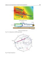
Flight Program . . . . . . . . . . . . . . . . . . . . . . . . . . . . . . . . . . . . . . . . . . . . . . . . . 189
References . . . . . . . . . . . . . . . . . . . . . . . . . . . . . . . . . . . . . . . . . . . . . . . . . . . . 192

13 Autonomous Vessels and Underwater Vehicles
13.1
13.2
13.3
13.4
13.5

165

215

Mobile Robot Simulation . . . . . . . . . . . . . . . . . . . . . . . . . . . . . . . . . . . . . . . . 215
EyeSim Simulation System . . . . . . . . . . . . . . . . . . . . . . . . . . . . . . . . . . . . . . . 216
Multiple Robot Simulation . . . . . . . . . . . . . . . . . . . . . . . . . . . . . . . . . . . . . . . 221
EyeSim Application. . . . . . . . . . . . . . . . . . . . . . . . . . . . . . . . . . . . . . . . . . . . . 222
EyeSim Environment and Parameter Files . . . . . . . . . . . . . . . . . . . . . . . . . . . 223
SubSim Simulation System . . . . . . . . . . . . . . . . . . . . . . . . . . . . . . . . . . . . . . . 228
Actuator and Sensor Models . . . . . . . . . . . . . . . . . . . . . . . . . . . . . . . . . . . . . . 230
SubSim Application. . . . . . . . . . . . . . . . . . . . . . . . . . . . . . . . . . . . . . . . . . . . . 232
SubSim Environment and Parameter Files . . . . . . . . . . . . . . . . . . . . . . . . . . . 234
References . . . . . . . . . . . . . . . . . . . . . . . . . . . . . . . . . . . . . . . . . . . . . . . . . . . . 237

PART III: MOBILE ROBOT APPLICATIONS
16 Localization and Navigation
16.1
16.2
16.3
16.4
16.5
16.6
16.7

241

Localization . . . . . . . . . . . . . . . . . . . . . . . . . . . . . . . . . . . . . . . . . . . . . . . . . . . 241
Probabilistic Localization . . . . . . . . . . . . . . . . . . . . . . . . . . . . . . . . . . . . . . . . 245
Coordinate Systems . . . . . . . . . . . . . . . . . . . . . . . . . . . . . . . . . . . . . . . . . . . . . 249
Environment Representation . . . . . . . . . . . . . . . . . . . . . . . . . . . . . . . . . . . . . . 251
Visibility Graph . . . . . . . . . . . . . . . . . . . . . . . . . . . . . . . . . . . . . . . . . . . . . . . . 253
Voronoi Diagram . . . . . . . . . . . . . . . . . . . . . . . . . . . . . . . . . . . . . . . . . . . . . . . 255
Potential Field Method . . . . . . . . . . . . . . . . . . . . . . . . . . . . . . . . . . . . . . . . . . 258

XIXI


Contents
16.8
16.9
16.10
16.11
16.12

Wandering Standpoint Algorithm . . . . . . . . . . . . . . . . . . . . . . . . . . . . . . . . . . 259
Bug Algorithm Family . . . . . . . . . . . . . . . . . . . . . . . . . . . . . . . . . . . . . . . . . . 260
Dijkstra’s Algorithm . . . . . . . . . . . . . . . . . . . . . . . . . . . . . . . . . . . . . . . . . . . . 263
A* Algorithm. . . . . . . . . . . . . . . . . . . . . . . . . . . . . . . . . . . . . . . . . . . . . . . . . . 267
References . . . . . . . . . . . . . . . . . . . . . . . . . . . . . . . . . . . . . . . . . . . . . . . . . . . . 268

17 Maze Exploration
17.1
17.2
17.3
17.4

18 Map Generation
18.1
18.2
18.3
18.4
18.5
18.6
18.7

18.8

XII

317

RoboCup and FIRA Competitions. . . . . . . . . . . . . . . . . . . . . . . . . . . . . . . . . . 317
Team Structure. . . . . . . . . . . . . . . . . . . . . . . . . . . . . . . . . . . . . . . . . . . . . . . . . 320
Mechanics and Actuators. . . . . . . . . . . . . . . . . . . . . . . . . . . . . . . . . . . . . . . . . 321
Sensing. . . . . . . . . . . . . . . . . . . . . . . . . . . . . . . . . . . . . . . . . . . . . . . . . . . . . . . 321
Image Processing . . . . . . . . . . . . . . . . . . . . . . . . . . . . . . . . . . . . . . . . . . . . . . . 323
Trajectory Planning . . . . . . . . . . . . . . . . . . . . . . . . . . . . . . . . . . . . . . . . . . . . . 325
References . . . . . . . . . . . . . . . . . . . . . . . . . . . . . . . . . . . . . . . . . . . . . . . . . . . . 330

21 Neural Networks
21.1
21.2
21.3
21.4
21.5
21.6

297

Camera Interface . . . . . . . . . . . . . . . . . . . . . . . . . . . . . . . . . . . . . . . . . . . . . . . 297
Auto-Brightness . . . . . . . . . . . . . . . . . . . . . . . . . . . . . . . . . . . . . . . . . . . . . . . . 299
Edge Detection. . . . . . . . . . . . . . . . . . . . . . . . . . . . . . . . . . . . . . . . . . . . . . . . . 300
Motion Detection . . . . . . . . . . . . . . . . . . . . . . . . . . . . . . . . . . . . . . . . . . . . . . . 302
Color Space . . . . . . . . . . . . . . . . . . . . . . . . . . . . . . . . . . . . . . . . . . . . . . . . . . . 303
Color Object Detection . . . . . . . . . . . . . . . . . . . . . . . . . . . . . . . . . . . . . . . . . . 305

Image Segmentation . . . . . . . . . . . . . . . . . . . . . . . . . . . . . . . . . . . . . . . . . . . . 310
Image Coordinates versus World Coordinates . . . . . . . . . . . . . . . . . . . . . . . . 312
References . . . . . . . . . . . . . . . . . . . . . . . . . . . . . . . . . . . . . . . . . . . . . . . . . . . . 314

20 Robot Soccer
20.1
20.2
20.3
20.4
20.5
20.6
20.7

283

Mapping Algorithm . . . . . . . . . . . . . . . . . . . . . . . . . . . . . . . . . . . . . . . . . . . . . 283
Data Representation. . . . . . . . . . . . . . . . . . . . . . . . . . . . . . . . . . . . . . . . . . . . . 285
Boundary-Following Algorithm . . . . . . . . . . . . . . . . . . . . . . . . . . . . . . . . . . . 286
Algorithm Execution . . . . . . . . . . . . . . . . . . . . . . . . . . . . . . . . . . . . . . . . . . . . 287
Simulation Experiments. . . . . . . . . . . . . . . . . . . . . . . . . . . . . . . . . . . . . . . . . . 289
Robot Experiments . . . . . . . . . . . . . . . . . . . . . . . . . . . . . . . . . . . . . . . . . . . . . 290
Results . . . . . . . . . . . . . . . . . . . . . . . . . . . . . . . . . . . . . . . . . . . . . . . . . . . . . . . 293
References . . . . . . . . . . . . . . . . . . . . . . . . . . . . . . . . . . . . . . . . . . . . . . . . . . . . 294

19 Real-Time Image Processing
19.1
19.2
19.3
19.4
19.5

19.6
19.7
19.8
19.9

271

Micro Mouse Contest . . . . . . . . . . . . . . . . . . . . . . . . . . . . . . . . . . . . . . . . . . . 271
Maze Exploration Algorithms . . . . . . . . . . . . . . . . . . . . . . . . . . . . . . . . . . . . . 273
Simulated versus Real Maze Program . . . . . . . . . . . . . . . . . . . . . . . . . . . . . . . 281
References . . . . . . . . . . . . . . . . . . . . . . . . . . . . . . . . . . . . . . . . . . . . . . . . . . . . 282

331

Neural Network Principles . . . . . . . . . . . . . . . . . . . . . . . . . . . . . . . . . . . . . . . 331
Feed-Forward Networks . . . . . . . . . . . . . . . . . . . . . . . . . . . . . . . . . . . . . . . . . 332
Backpropagation . . . . . . . . . . . . . . . . . . . . . . . . . . . . . . . . . . . . . . . . . . . . . . . 337
Neural Network Examples. . . . . . . . . . . . . . . . . . . . . . . . . . . . . . . . . . . . . . . . 342
Neural Controller . . . . . . . . . . . . . . . . . . . . . . . . . . . . . . . . . . . . . . . . . . . . . . . 343
References . . . . . . . . . . . . . . . . . . . . . . . . . . . . . . . . . . . . . . . . . . . . . . . . . . . . 344


Contents

22 Genetic Algorithms
22.1
22.2
22.3
22.4
22.5

22.6
22.7

Genetic Algorithm Principles . . . . . . . . . . . . . . . . . . . . . . . . . . . . . . . . . . . . . 348
Genetic Operators . . . . . . . . . . . . . . . . . . . . . . . . . . . . . . . . . . . . . . . . . . . . . . 350
Applications to Robot Control. . . . . . . . . . . . . . . . . . . . . . . . . . . . . . . . . . . . . 352
Example Evolution . . . . . . . . . . . . . . . . . . . . . . . . . . . . . . . . . . . . . . . . . . . . . 353
Implementation of Genetic Algorithms . . . . . . . . . . . . . . . . . . . . . . . . . . . . . . 357
Starman . . . . . . . . . . . . . . . . . . . . . . . . . . . . . . . . . . . . . . . . . . . . . . . . . . . . . . 361
References . . . . . . . . . . . . . . . . . . . . . . . . . . . . . . . . . . . . . . . . . . . . . . . . . . . . 363

23 Genetic Programming
23.1
23.2
23.3
23.4
23.5
23.6
23.7

403

Splines . . . . . . . . . . . . . . . . . . . . . . . . . . . . . . . . . . . . . . . . . . . . . . . . . . . . . . . 403
Control Algorithm . . . . . . . . . . . . . . . . . . . . . . . . . . . . . . . . . . . . . . . . . . . . . . 404
Incorporating Feedback . . . . . . . . . . . . . . . . . . . . . . . . . . . . . . . . . . . . . . . . . . 406
Controller Evolution . . . . . . . . . . . . . . . . . . . . . . . . . . . . . . . . . . . . . . . . . . . . 407
Controller Assessment . . . . . . . . . . . . . . . . . . . . . . . . . . . . . . . . . . . . . . . . . . . 409
Evolved Gaits. . . . . . . . . . . . . . . . . . . . . . . . . . . . . . . . . . . . . . . . . . . . . . . . . . 410
References . . . . . . . . . . . . . . . . . . . . . . . . . . . . . . . . . . . . . . . . . . . . . . . . . . . . 413

26 Automotive Systems
26.1
26.2
26.3
26.4
26.5
26.6
26.7
26.8

383

Software Architecture . . . . . . . . . . . . . . . . . . . . . . . . . . . . . . . . . . . . . . . . . . . 383
Behavior-Based Robotics . . . . . . . . . . . . . . . . . . . . . . . . . . . . . . . . . . . . . . . . 384
Behavior-Based Applications . . . . . . . . . . . . . . . . . . . . . . . . . . . . . . . . . . . . . 387
Behavior Framework . . . . . . . . . . . . . . . . . . . . . . . . . . . . . . . . . . . . . . . . . . . . 388
Adaptive Controller . . . . . . . . . . . . . . . . . . . . . . . . . . . . . . . . . . . . . . . . . . . . . 391
Tracking Problem . . . . . . . . . . . . . . . . . . . . . . . . . . . . . . . . . . . . . . . . . . . . . . 395
Neural Network Controller . . . . . . . . . . . . . . . . . . . . . . . . . . . . . . . . . . . . . . . 396
Experiments . . . . . . . . . . . . . . . . . . . . . . . . . . . . . . . . . . . . . . . . . . . . . . . . . . . 398
References . . . . . . . . . . . . . . . . . . . . . . . . . . . . . . . . . . . . . . . . . . . . . . . . . . . . 400

25 Evolution of Walking Gaits
25.1
25.2
25.3
25.4
25.5
25.6
25.7

365

Concepts and Applications . . . . . . . . . . . . . . . . . . . . . . . . . . . . . . . . . . . . . . . 365
Lisp . . . . . . . . . . . . . . . . . . . . . . . . . . . . . . . . . . . . . . . . . . . . . . . . . . . . . . . . . 367
Genetic Operators . . . . . . . . . . . . . . . . . . . . . . . . . . . . . . . . . . . . . . . . . . . . . . 371
Evolution . . . . . . . . . . . . . . . . . . . . . . . . . . . . . . . . . . . . . . . . . . . . . . . . . . . . . 373
Tracking Problem . . . . . . . . . . . . . . . . . . . . . . . . . . . . . . . . . . . . . . . . . . . . . . 374
Evolution of Tracking Behavior . . . . . . . . . . . . . . . . . . . . . . . . . . . . . . . . . . . 377
References . . . . . . . . . . . . . . . . . . . . . . . . . . . . . . . . . . . . . . . . . . . . . . . . . . . . 381

24 Behavior-Based Systems
24.1
24.2
24.3
24.4
24.5
24.6
24.7
24.8
24.9

347

415

Autonomous Automobiles . . . . . . . . . . . . . . . . . . . . . . . . . . . . . . . . . . . . . . . . 415
Automobile Conversion for Autonomous Driving . . . . . . . . . . . . . . . . . . . . . 418
Computer Vision for Driver-Assistance Systems . . . . . . . . . . . . . . . . . . . . . . 420
Image Processing Framework . . . . . . . . . . . . . . . . . . . . . . . . . . . . . . . . . . . . . 421

Lane Detection. . . . . . . . . . . . . . . . . . . . . . . . . . . . . . . . . . . . . . . . . . . . . . . . . 422
Vehicle Recognition and Tracking . . . . . . . . . . . . . . . . . . . . . . . . . . . . . . . . . 429
Automatic Parking . . . . . . . . . . . . . . . . . . . . . . . . . . . . . . . . . . . . . . . . . . . . . . 433
References . . . . . . . . . . . . . . . . . . . . . . . . . . . . . . . . . . . . . . . . . . . . . . . . . . . . 436

27 Outlook

439
XIIIXIII


Contents

APPENDICES
A
B
C
D
E
F

Programming Tools . . . . . . . . . . . . . . . . . . . . . . . . . . . . . . . . . . . . . . . . . . . . . . . . . . 443
RoBIOS Operating System . . . . . . . . . . . . . . . . . . . . . . . . . . . . . . . . . . . . . . . . . . . . 453
Hardware Description Table . . . . . . . . . . . . . . . . . . . . . . . . . . . . . . . . . . . . . . . . . . . 495
Hardware Specification . . . . . . . . . . . . . . . . . . . . . . . . . . . . . . . . . . . . . . . . . . . . . . . 511
Laboratories . . . . . . . . . . . . . . . . . . . . . . . . . . . . . . . . . . . . . . . . . . . . . . . . . . . . . . . . 519
Solutions. . . . . . . . . . . . . . . . . . . . . . . . . . . . . . . . . . . . . . . . . . . . . . . . . . . . . . . . . . . 529

Index

XIV

533


ROBOTS AND
C
ONTROLLERS
...................................
.........
obotics has come a long way. Especially for mobile robots, a similar
trend is happening as we have seen for computer systems: the transition from mainframe computing via workstations to PCs, which will
probably continue with handheld devices for many applications. In the past,
mobile robots were controlled by heavy, large, and expensive computer systems that could not be carried and had to be linked via cable or wireless
devices. Today, however, we can build small mobile robots with numerous
actuators and sensors that are controlled by inexpensive, small, and light
embedded computer systems that are carried on-board the robot.
There has been a tremendous increase of interest in mobile robots. Not just
as interesting toys or inspired by science fiction stories or movies [Asimov
1950], but as a perfect tool for engineering education, mobile robots are used
today at almost all universities in undergraduate and graduate courses in Computer Science/Computer Engineering, Information Technology, Cybernetics,
Electrical Engineering, Mechanical Engineering, and Mechatronics.
What are the advantages of using mobile robot systems as opposed to traditional ways of education, for example mathematical models or computer simulation?
First of all, a robot is a tangible, self-contained piece of real-world hardware. Students can relate to a robot much better than to a piece of software.
Tasks to be solved involving a robot are of a practical nature and directly
“make sense” to students, much more so than, for example, the inevitable comparison of sorting algorithms.
Secondly, all problems involving “real-world hardware” such as a robot, are
in many ways harder than solving a theoretical problem. The “perfect world”
which often is the realm of pure software systems does not exist here. Any
actuator can only be positioned to a certain degree of accuracy, and all sensors

have intrinsic reading errors and certain limitations. Therefore, a working
robot program will be much more than just a logic solution coded in software.
33


1

Robots and Controllers
It will be a robust system that takes into account and overcomes inaccuracies
and imperfections. In summary: a valid engineering approach to a typical
(industrial) problem.
Third and finally, mobile robot programming is enjoyable and an inspiration to students. The fact that there is a moving system whose behavior can be
specified by a piece of software is a challenge. This can even be amplified by
introducing robot competitions where two teams of robots compete in solving
a particular task [Bräunl 1999] – achieving a goal with autonomously operating robots, not remote controlled destructive “robot wars”.

1.1 Mobile Robots
Since the foundation of the Mobile Robot Lab by the author at The University
of Western Australia in 1998, we have developed a number of mobile robots,
including wheeled, tracked, legged, flying, and underwater robots. We call
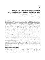
these robots the “EyeBot family” of mobile robots (Figure 1.1), because they
are all using the same embedded controller “EyeCon” (EyeBot controller, see
the following section).

Figure 1.1: Some members of the EyeBot family of mobile robots
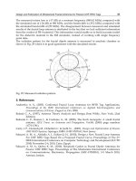
The simplest case of mobile robots are wheeled robots, as shown in Figure
1.2. Wheeled robots comprise one or more driven wheels (drawn solid in the
figure) and have optional passive or caster wheels (drawn hollow) and possibly steered wheels (drawn inside a circle). Most designs require two motors for
driving (and steering) a mobile robot.
The design on the left-hand side of Figure 1.2 has a single driven wheel that

is also steered. It requires two motors, one for driving the wheel and one for
turning. The advantage of this design is that the driving and turning actions
4


Mobile Robots

Figure 1.2: Wheeled robots
have been completely separated by using two different motors. Therefore, the
control software for driving curves will be very simple. A disadvantage of this
design is that the robot cannot turn on the spot, since the driven wheel is not
located at its center.
The robot design in the middle of Figure 1.2 is called “differential drive”
and is one of the most commonly used mobile robot designs. The combination
of two driven wheels allows the robot to be driven straight, in a curve, or to
turn on the spot. The translation between driving commands, for example a
curve of a given radius, and the corresponding wheel speeds has to be done
using software. Another advantage of this design is that motors and wheels are
in fixed positions and do not need to be turned as in the previous design. This
simplifies the robot mechanics design considerably.
Finally, on the right-hand side of Figure 1.2 is the so-called “Ackermann
Steering”, which is the standard drive and steering system of a rear-driven passenger car. We have one motor for driving both rear wheels via a differential
box and one motor for combined steering of both front wheels.
It is interesting to note that all of these different mobile robot designs
require two motors in total for driving and steering.
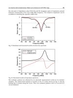
A special case of a wheeled robot is the omni-directional “Mecanum drive”
robot in Figure 1.3, left. It uses four driven wheels with a special wheel design
and will be discussed in more detail in a later chapter.

Figure 1.3: Omni-directional, tracked, and walking robots

One disadvantage of all wheeled robots is that they require a street or some
sort of flat surface for driving. Tracked robots (see Figure 1.3, middle) are
more flexible and can navigate over rough terrain. However, they cannot navigate as accurately as a wheeled robot. Tracked robots also need two motors,
one for each track.
5


1

Braitenberg
vehicles

Robots and Controllers
Legged robots (see Figure 1.3, right) are the final category of land-based
mobile robots. Like tracked robots, they can navigate over rough terrain or
climb up and down stairs, for example. There are many different designs for
legged robots, depending on their number of legs. The general rule is: the more
legs, the easier to balance. For example, the six-legged robot shown in the figure can be operated in such a way that three legs are always on the ground
while three legs are in the air. The robot will be stable at all times, resting on a
tripod formed from the three legs currently on the ground – provided its center
of mass falls in the triangle described by these three legs. The less legs a robot
has, the more complex it gets to balance and walk, for example a robot with
only four legs needs to be carefully controlled, in order not to fall over. A
biped (two-legged) robot cannot play the same trick with a supporting triangle,
since that requires at least three legs. So other techniques for balancing need to
be employed, as is discussed in greater detail in Chapter 11. Legged robots
usually require two or more motors (“degrees of freedom”) per leg, so a sixlegged robot requires at least 12 motors. Many biped robot designs have five
or more motors per leg, which results in a rather large total number of degrees
of freedom and also in considerable weight and cost.
A very interesting conceptual abstraction of actuators, sensors, and robot

control is the vehicles described by Braitenberg [Braitenberg 1984]. In one
example, we have a simple interaction between motors and light sensors. If a
light sensor is activated by a light source, it will proportionally increase the
speed of the motor it is linked to.

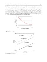
Figure 1.4: Braitenberg vehicles avoiding light (phototroph)
In Figure 1.4 our robot has two light sensors, one on the front left, one on
the front right. The left light sensor is linked to the left motor, the right sensor
to the right motor. If a light source appears in front of the robot, it will start
driving toward it, because both sensors will activate both motors. However,
what happens if the robot gets closer to the light source and goes slightly off
course? In this case, one of the sensors will be closer to the light source (the
left sensor in the figure), and therefore one of the motors (the left motor in the
figure) will become faster than the other. This will result in a curve trajectory
of our robot and it will miss the light source.
6


Embedded Controllers

Figure 1.5: Braitenberg vehicles searching light (photovore)
Figure 1.5 shows a very similar scenario of Braitenberg vehicles. However,
here we have linked the left sensor to the right motor and the right sensor to the
left motor. If we conduct the same experiment as before, again the robot will
start driving when encountering a light source. But when it gets closer and also
slightly off course (veering to the right in the figure), the left sensor will now
receive more light and therefore accelerate the right motor. This will result in a
left curve, so the robot is brought back on track to find the light source.
Braitenberg vehicles are only a limited abstraction of robots. However, a
number of control concepts can easily be demonstrated by using them.

1.2 Embedded Controllers
The centerpiece of all our robot designs is a small and versatile embedded controller that each robot carries on-board. We called it the “EyeCon” (EyeBot
controller, Figure 1.6), since its chief specification was to provide an interface
for a digital camera in order to drive a mobile robot using on-board image
processing [Bräunl 2001].

Figure 1.6: EyeCon, front and with camera attached

7


1

Robots and Controllers
The EyeCon is a small, light, and fully self-contained embedded controller.
It combines a 32bit CPU with a number of standard interfaces and drivers for
DC motors, servos, several types of sensors, plus of course a digital color camera. Unlike most other controllers, the EyeCon comes with a complete built-in
user interface: it comprises a large graphics display for displaying text messages and graphics, as well as four user input buttons. Also, a microphone and
a speaker are included. The main characteristics of the EyeCon are:

EyeCon specs

•
•
•
•
•
•
•

•
•
•
•
•
•
•
•
•
•
•
•

25MHz 32bit controller (Motorola M68332)
1MB RAM, extendable to 2MB
512KB ROM (for system + user programs)
1 Parallel port
3 Serial ports (1 at V24, 2 at TTL)
8 Digital inputs
8 Digital outputs
16 Timing processor unit inputs/outputs
8 Analog inputs
Single compact PCB
Interface for color and grayscale camera
Large graphics LCD (128× 64 pixels)
4 input buttons
Reset button
Power switch
Audio output
• Piezo speaker

• Adapter and volume potentiometer for external speaker
Microphone for audio input
Battery level indication
Connectors for actuators and sensors:
• Digital camera
• 2 DC motors with encoders
• 12 Servos
• 6 Infrared sensors
• 6 Free analog inputs

One of the biggest achievements in designing hardware and software for the
EyeCon embedded controller was interfacing to a digital camera to allow onboard real-time image processing. We started with grayscale and color Connectix “QuickCam” camera modules for which interface specifications were
available. However, this was no longer the case for successor models and it is
virtually impossible to interface a camera if the manufacturer does not disclose
the protocol. This lead us to develop our own camera module “EyeCam” using
low resolution CMOS sensor chips. The current design includes a FIFO hardware buffer to increase the throughput of image data.
A number of simpler robots use only 8bit controllers [Jones, Flynn, Seiger
1999]. However, the major advantage of using a 32bit controller versus an 8bit
controller is not just its higher CPU frequency (about 25 times faster) and
8


Embedded Controllers
wider word format (4 times), but the ability to use standard off-the-shelf C and
C++ compilers. Compilation makes program execution about 10 times faster
than interpretation, so in total this results in a system that is 1,000 times faster.
We are using the GNU C/C++ cross-compiler for compiling both the operating
system and user application programs under Linux or Windows. This compiler
is the industry standard and highly reliable. It is not comparable with any of
the C-subset interpreters available.

The EyeCon embedded controller runs our own “RoBIOS” (Robot Basic
Input Output System) operating system that resides in the controller’s flashROM. This allows a very simple upgrade of a controller by simply downloading a new system file. It only requires a few seconds and no extra equipment,
since both the Motorola background debugger circuitry and the writeable
flash-ROM are already integrated into the controller.
RoBIOS combines a small monitor program for loading, storing, and executing programs with a library of user functions that control the operation of
all on-board and off-board devices (see Appendix B.5). The library functions
include displaying text/graphics on the LCD, reading push-button status, reading sensor data, reading digital images, reading robot position data, driving
motors, v-omega (vω) driving interface, etc. Included also is a thread-based
multitasking system with semaphores for synchronization. The RoBIOS operating system is discussed in more detail in Chapter B.
Another important part of the EyeCon’s operating system is the HDT
(Hardware Description Table). This is a system table that can be loaded to
flash-ROM independent of the RoBIOS version. So it is possible to change the
system configuration by changing HDT entries, without touching the RoBIOS
operating system. RoBIOS can display the current HDT and allows selection
and testing of each system component listed (for example an infrared sensor or
a DC motor) by component-specific testing routines.
Figure 1.7 from [InroSoft 2006], the commercial producer of the EyeCon
controller, shows hardware schematics. Framed by the address and data buses
on the top and the chip-select lines on the bottom are the main system components ROM, RAM, and latches for digital I/O. The LCD module is memory
mapped, and therefore looks like a special RAM chip in the schematics.
Optional parts like the RAM extension are shaded in this diagram. The digital
camera can be interfaced through the parallel port or the optional FIFO buffer.
While the Motorola M68332 CPU on the left already provides one serial port,
we are using an ST16C552 to add a parallel port and two further serial ports to
the EyeCon system. Serial-1 is converted to V24 level (range +12V to –12V)
with the help of a MAX232 chip. This allows us to link this serial port directly
to any other device, such as a PC, Macintosh, or workstation for program
download. The other two serial ports, Serial-2 and Serial-3, stay at TTL level
(+5V) for linking other TTL-level communication hardware, such as the wireless module for Serial-2 and the IRDA wireless infrared module for Serial-3.
A number of CPU ports are hardwired to EyeCon system components; all

others can be freely assigned to sensors or actuators. By using the HDT, these
assignments can be defined in a structured way and are transparent to the user
9


1

Robots and Controllers

© InroSoft, Thomas Bräunl 2006

Figure 1.7: EyeCon schematics
program. The on-board motor controllers and feedback encoders utilize the
lower TPU channels plus some pins from the CPU port E, while the speaker
uses the highest TPU channel. Twelve TPU channels are provided with matching connectors for servos, i.e. model car/plane motors with pulse width modulation (PWM) control, so they can simply be plugged in and immediately operated. The input keys are linked to CPU port F, while infrared distance sensors
(PSDs, position sensitive devices) can be linked to either port E or some of the
digital inputs.
An eight-line analog to digital (A/D) converter is directly linked to the
CPU. One of its channels is used for the microphone, and one is used for the
battery status. The remaining six channels are free and can be used for connecting analog sensors.

1.3 Interfaces
A number of interfaces are available on most embedded systems. These are
digital inputs, digital outputs, and analog inputs. Analog outputs are not
always required and would also need additional amplifiers to drive any actuators. Instead, DC motors are usually driven by using a digital output line and a
pulsing technique called “pulse width modulation” (PWM). See Chapter 4 for
10


Interfaces

video out
camera connector IR receiver
serial 1
serial 2

graphics LCD

reset button
power switch
speaker microphone

input buttons

parallel port
motors and encoders (2)
background debugger
analog inputs
digital I/O
servos (14)

power

PSD (6) serial 3

Figure 1.8: EyeCon controller M5, front and back
details. The Motorola M68332 microcontroller already provides a number of
digital I/O lines, grouped together in ports. We are utilizing these CPU ports as

11

1

Robots and Controllers
can be seen in the schematics diagram Figure 1.7, but also provide additional
digital I/O pins through latches.
Most important is the M68332’s TPU. This is basically a second CPU integrated on the same chip, but specialized to timing tasks. It simplifies tremendously many time-related functions, like periodic signal generation or pulse
counting, which are frequently required for robotics applications.
Figure 1.8 shows the EyeCon board with all its components and interface
connections from the front and back. Our design objective was to make the
construction of a robot around the EyeCon as simple as possible. Most interface connectors allow direct plug-in of hardware components. No adapters or
special cables are required to plug servos, DC motors, or PSD sensors into the
EyeCon. Only the HDT software needs to be updated by simply downloading
the new configuration from a PC; then each user program can access the new
hardware.
The parallel port and the three serial ports are standard ports and can be
used to link to a host system, other controllers, or complex sensors/actuators.
Serial port 1 operates at V24 level, while the other two serial ports operate at
TTL level.
The Motorola background debugger (BDM) is a special feature of the
M68332 controller. Additional circuitry is included in the EyeCon, so only a
cable is required to activate the BDM from a host PC. The BDM can be used to
debug an assembly program using breakpoints, single step, and memory or
register display. It can also be used to initialize the flash-ROM if a new chip is
inserted or the operating system has been wiped by accident.

Figure 1.9: EyeBox units

12

Operating System
At The University of Western Australia, we are using a stand-alone, boxed
version of the EyeCon controller (“EyeBox” Figure 1.9) for lab experiments in
the Embedded Systems course. They are used for the first block of lab experiments until we switch to the EyeBot Labcars (Figure 8.5). See Appendix E for
a collection of lab experiments.

1.4 Operating System
Embedded systems can have anything between a complex real-time operating
system, such as Linux, or just the application program with no operating system, whatsoever. It all depends on the intended application area. For the EyeCon controller, we developed our own operating system RoBIOS (Robot Basic
Input Output System), which is a very lean real-time operating system that
provides a monitor program as user interface, system functions (including
multithreading, semaphores, timers), plus a comprehensive device driver
library for all kinds of robotics and embedded systems applications. This
includes serial/parallel communication, DC motors, servos, various sensors,
graphics/text output, and input buttons. Details are listed in Appendix B.5.
User input/output

RoBIOS
Monitor program

User program

RoBIOS Operating system + Library functions
HDT
Hardware

Robot mechanics,
actuators, and sensors

Figure 1.10: RoBIOS structure
The RoBIOS monitor program starts at power-up and provides a comprehensive control interface to download and run programs, load and store programs in flash-ROM, test system components, and to set a number of system
parameters. An additional system component, independent of RoBIOS, is the
13