Đánh giá và mô phỏng các hệ số đàn hồi đa tintinh thể hỗn độn tt tiếng anh
Bạn đang xem bản rút gọn của tài liệu. Xem và tải ngay bản đầy đủ của tài liệu tại đây (1.8 MB, 27 trang )
MINISTRY OF EDUCATION
ANDTRAINING
VIETNAM ACADEMY OF
SCIENCE AND TECHNOLOGY
GRADUATE UNIVERSITY SCIENCE AND TECHNOLOGY
---------------------------
VUONG THI MY HANH
ESTIMATES AND SIMULATIONS FOR THE ELASTIC
MODULI OF RANDOM POLYCRYSTALS
Major: Mechanics of Solid
Code: 9440107
SUMARY OF DOCTORAL THESIS IN MECHANICS
HA NOI - 2020
The thesis has been completed at: Graduate University Science and
Technology -Vietnam Academy of Science and Technology.
Supervisor 1: Prof. DrSc. Pham Duc Chinh
Supervisor 2 : Dr. Le Hoai Chau
Reviewer 1: Prof. Dr. Pham Chi Vinh
Reviewer 2: Assoc. Prof. Dr. La Duc Viet
Reviewer 3: Assoc. Prof. Dr. Tran Bao Viet
Thesis is defended at Graduate University Scienc and TechnologyVietnam Academy of Science and Technology at ...: ..., on ... / ... / 2020
Hardcopy of the thesis be found at:
- Library of Graduate University Science and Technology
- Vietnam national library
1
PREFACE
1. Reason of choosing the thesis
a. Objective reason
Polycrystalline materials are being used extensively in all
areas of human life. The study of elastic coefficients for this
material yields many analytical results: Voigt, Ruess, Hill,
Hashin-Strikman, Pham Duc Chinh ... However, the finite
element method (FEM) results are not surffice for comparison.
The question is: are these estimates the best, how to calculate by
the FEM, how the FEM results compared to these estimates ...
b. Subjective reason
Homogenization of materials is a long-term research field of
supervisor Pham Duc Chinh and Material Mechanics team with
many published results. The PhD candidate completed the
master's thesis on homogenization of thermal conductivity for
isotropic composite materials. Therefore, author has selected
the topic "Estimates and simulation for the elastic moduli of
random polycrystals " as the research thesis.
2. Aim, research method of the thesis
a. Aim: to find better estimates, compare results of analytic
method and FEM.
b. Method: using energy principles and applying analytical and
numerical methods simultaneously.
3. Research subject and scope of the thesis
a. Subject: macroscopic elastic moduli of random polycrystals.
b. Scope: For estimates, thesis considers d- dimensional
polyscrystals; For simulation, thesis only considers 2D
polyscrystals with hexagonal shape of.
2
4. New contributions of the thesis
a. Theory: Generalized polarization fields, estimates and
specific calculation results for elastic moduli of d-dimensional
polyscrystals are new and better than the previous estimates.
b. Numerical simulation: Large-scale FEM results for elastic
moduli of 2D square, orthorhombic and tetragonal polycrystals
for comparisons with the bounds are new.
5. Thesis layout
Chapter 1 presents the development history and research
methods of the previous authors. Chapter 2 constructs general
estimates for macroscopic elastic moduli. Chapter 3 applies
Chapter 2 results to 2D and 3D polycrystals; calculates and
compares thesis estimates with V-R, HS, PĐC, SC estimates.
Chapter 4 applies FEM to simulate values of 2D polycrystal
macroscopic elastic moduli, compares with analytical results.
CHAPTER 1: OVERVIEW
1.1. Overview of polycrystaline materials
Polycrystalline materials are aggregates of large numbers of
individual crystals bonded perfectly together.
Figure 1.2: Random polycrystalline materials model
1.2. Research history of macroscopic elastic moduli
1.2.1. Outline the process of developing research field
Common approach is using energy priciples, statistical isotropy
and symmetric cell hypotheses have been applied to narrow the
bounds of estimates from the first order to the second order and
3
the third order ones. Experimental data shows that the values of
macroscopic properties concentrate within higher order bounds.
Therefore, third-order estimates are the best ones for the
macroscopic properties of polycrystals as well as composites.
1.2.2. Typical estimates
a. Voigt- Ruess- Hill estimate (first order)
k eff , eff :
macroscopic
bulk and
shear
elastic
moduli;
kV , V , kR , R : Voigt, Reuss estimates; Cijkl , Sijkl (i, j, k , l 1, d )
are the stiffness and compliant elastic tensors of α- orientation
crystal, respectively:
kV
1
1
1
Ciijj ; V 2
Cijij Ciijj
d2
d d 2
d
kR Siijj
1
; R
(1.1)
4
1
Sijij Siijj
2
d
d d 2
1
kV k eff kR ; V eff R
(1.2)
(1.3)
b. Hashin- Strikman estimate (second order)
HS used new variatinonal principle and polar field to buils
new estimates better than the Hill ones. In cubic case, HS
L
U
estimates for bulk uper k HS
and lower bound k HS
:
U
L
kHS
kHS
kV kR
1
2C11 2C11 C33
9
L
HS estimates for shear uper UHS and lower bounds HS
:
L
UHS P (C,k eff , 0UHS ) , HS
P (C,k eff , 0LHS ) ,
P (C, k 0 , 0 ) 5
C
11
C12 2* (C44 * )
3(C11 C12 ) 4C44 10*
* ,
(1.5)
4
* 0
9k0 80
C C12
, 0UHS max 11
, C44 ,
2
6k0 120
C11 C12
, C44 .
2
0LHS min
(1.8)
c. Pham Duc Chinh estimate (third order)
Using HS-type polarization trial fields, but coming derectly
from classical minimum energy and complementary energy
principles, PDC added three-point correlation parameters
A , B and succeded in constructing tighter bounds. PDC
estimates have short forms for spherical cell polycrystals:
9 k0 8 0
4
(1.10)
Cij*kl Tijkl (k* , * );k* 0 ; * 0
3
6k0 120
ε0 : Ceff : ε 0 ε 0 : C * )1
1
σ 0 : (Ceff )1 : σ 0 σ 0 : C * )1
C* : ε 0 , C0 C
1
C*
1
0
1
: σ0 , C C
(1.24)
1
(1.26)
d. Self- consistent value(SC)
SC value is the solution C0 of the equation:
C0
1
* 1
C
C*
(1.27)
Advantages: SC values are calculated simply and quickly;
Disadvantages: they are valid only for perfect material model
and has many deviations, so thesis only uses it for reference.
1.3. General research method
1.3.1. Analytical method
The problem is solved by finding extremums of energy
functions on RVE domain. Specifically: we choose one or more
possible test fields for deformations and stresses, put in
mechanical equations with constraints, and transform them to
5
get evaluations. This method is the traditional variational one
that V-R, HS, PDC used.
1.3.2. Numerical method
FEM is commonly used, the basic steps are: random crystal
orientation gereration, meshing RVE, setting stiffness matrix,
equations describing the material balance, applying conditions,
solving systems of equations to get the node displacements,
deformation, stress, ... caculating effective elastic coefficients.
1.4. Conclusion of chapter 1
Studying elastic moduli of polycrystalline materials has high
scientific and practical significance. The analytical results have
been developed well, but the FEM results are few. Therefore, in
this thesis PhD will use both analytical and numerical methods
in solving this problem, compare them with each other and give
specific conclusions.
CHAPTER 2: ESTIMATES FOR ELASTIC MODULI OF
D- DIMENSIONAL RANDOM POLYCRYSTALS
This chapter uses analytic methods to construct general
upper and lower bounds for the bulk and shear elastic moduli of
d-dimensional polycrystals. Conclusions for these estimates are
presented at the end of this chapter.
2.1. Scientific basis
2.1.1. Elastic coefficients of single crystal
Elastic properties of single crystals are anisotropic and often
used by the 2 index-Voigt notation C Cmn , S Smn ,
m, n 1,6 or 4 index C Cijkl
, S Sijkl , i, j, k , l 1, d .
2.1.2. Elastic coeficicents of polycrystals
Elastic moduli are determined by the folowing fomulae:
6
a. Hooke's law
Average stress field and strain field are related:
σ Ceff : ε
(2.22)
b. Minimum energy princilple ( ε is compatible)
Wε ε0 : Ceff : ε0 inf 0 ε : C : εdx
ε ε
(2.29)
V
c. Minimum complementary energy princilple( σ is balanced)
Wσ σ 0 : Ceff
1
: σ 0 inf 0 σ : C1 : σdx
σ σ
(2.34)
V
2.2. Bulk elastic modulus of d-dimensional polycrystals
2.2.1. Begining equations
We consider RVE has volume V=1, v is corresponding
volume ratio of V V . Three-point correlation parameters:
A ij ij dx , ij ,ij
V
1
v
,ijkl
B ijkl
ijkl dx , ijkl
V
,ij
dx ,
V
1
v
,ijkl
dx .
(2.50)
V
, are harmonic and biharmonic functions. Geometric
parameters f1, f3, g1, g3 are restricted by:
f1 f3
d 1
(d 1)(d 3)
, g1 g3
d(d 2)
d
(2.52)
6
d2 1
6
d 1
f1
g1
f1
f1 0 ,
d4
(d 2)(d 4)
d4
d
(2.54)
2.2.2. Upper bound of bulk elastic modulus
HS polarization trial field has form:
ij
3k0 0
0 (3k0 40 )
p
kl
,ijkl
1
0
p (i )
m
,j m
(2.55)
7
This field has only 2 free coefficients k0 , 0 . Refering to HS
field, PDC ’s thesis, PhD selects diffirent general polar fields
for upper and lower bounds, specifically with the upper bound:
ij
n
1
1
ij ε0 aik ,kj ajk,ki bakl ,ijkl
d
1 2
(2.56)
ε 0 is volumetric strain field; a aij are free scalar constants
n
restricted by
v a 0 ;
0 b 2 is free parameter.
1
After putting trial strain field in to minimum energy expression,
transforming it, we have:
W kV ε0
2
2ε0
n
v CK : a
1
n
v a : A : a
(2.60)
1
bkV
1
2b
A
CK CijK Cijkk 2 1
, A C pq
ij
d
2
d
2
d
A
C pq
C 'pqA Dpq ,
1
1
Cikjl C jkil B2 Ciipp kl Cklppij B3
2
2
1
1
Cipjp kl Ckplpij B4 Cipkp jl C jpkpil C jplpik Ciplp jk B5
2
4
1
Cikpp jl C jlpp ik C jkpp il Cilpp jk B6 ,
4
1
Dijkl ij kl D1 ik jl il jk D2 ,
2
2
D1 kV V f3 F1 g3G1 V f3 F2 g3G2
d
Cij' Akl Cijkl B1
d2 d 2
dkV f3 F3 g3G3 kV
V f3 F4 g3G4 ,
d
8
d 1 d 3
d 1
b2
F7
G7
kV ,
d
d d 2
d 2 2
d 2
D2 2V f3 F1 g3G1 kV
V f3 F2 g3G2
d
d2 d 2
d 1
kV
V f3 F5 g3G5 dkV f3 F6 g3G6
F8 ,
d
d
2
d 1 d 3 ,
1
2b
G8 B1 2 1
f1 F1 g1 G1 ,
d d 2
d d 2
B2 f1 F2 g1 G2 , B3
4b2
2b
f1 F3 g1 G3
d 2 d 2 d 2 d 2 2
B4 f1 F4 g1 G4 , B5 f1 F5 g1 G5 , B6 f1 F6 g1 G6
(2.61)
Optimizing (2.60) over the free variables aij restricted by
(2.59), using Lagrange multiplier method, we recive:
k eff k Ud C, f1 , g1 , b , k Ud kV CK : A-1
A-1
1
: A-1 : CK
CK : A1 : CK
:
(2.63)
Now optimizing (2.63) over the remaining parameter b, shape
parameters f1, g1 restricted by (2.52), (2.54), we obtain the upper
estimate:
k eff max min K Ud C, f1 , g1 , b
f1 , g1
b
(2.64)
Here we choose minimum over b because: trial strain field
admissible at all the values of b, so we choose the b in order to
ensure the smallest bulk modulus.
Choose maximum over f1, g1: these are two parameters
representing the geometry of polycrystals, so select the biggest
values to ensure the upper bound.
9
2.2.3. Lower bound of bulk elastic modulus
Similarly, we select general trial stress field:
n
ij ij 0 aik ,kj a jk,ki b 1 ij akl ,kl
1
aij bakl ,ijkl
(2.65)
n
v a 0 ;
where a are free scalar constants restricted by
1
I is the geometric indicator function of α-phase.
Putting this trial feld in to minimum complemantary energy
expression , optimizing over variables aij , b, f1, g1 restricted,
we obtain the lower bound:
k eff min max K Ld C, f1 , g1 , K Ld kR1 CK : A-1
f1 , g1 b
1
A-1
: A-1 : CK
CK : A1 : CK
:
1
(2.73)
2.3. Shear elastic modulus of d-dimensional polycrystals
2.3.1. Upper bound of shear elastic modulus
General trial strain field has form:
1
aik,kj ajk,ki bakl ,ijkl
1 2
Similarly, we have upper bound:
eff max min Ud C, f1 , g1 , b ,
n
ij ij0
f1 , g1
Ud V
A-1
(2.75)
b
1
1
T
-1
M ijij M iijj , M CM : A
3
d d 2
1
2
: A-1 : CM
CTM : A1 : CM
2.3.2. Lower bound of shear elastic modulus
We choose general trial stress field as:
:
(2.79)
10
n
ij ij0 aik ,kj a jk,ki b 1 ij akl ,kl
1
aij bakl ,ijkl
(2.80)
Transforming it silmilarly, we obtain:
eff min max Ld C, f1 , g1 ,
f1 , g1
b
1
Ld
2
1
R1 M ijij M iijj , M M ijkl CTM : A-1
5
3
A-1
1
: A-1 : CM
CTM : A1 : CM
:
(2.84)
2.4. Conclusion of chapter 2
Starting from energy principles, with trial fields being more
general than HS, thesis have built new estimates for elastic
moduli of d-dimensional polycrystalline materials:
This estimates are complexly dependent on the geometric
parameters f1, g1 and component elastic coefficients Cij .
Without these geometric informations, the estimates are V-R
bounds. The second term in our evaluation expressions makes
the results of the thesis better.
CHAPTER 3: ESTIMATES FOR EFFECTIVE ELASTIC
MODULI OF SPECIFIC POLYCRYSTAL CLASSES
This chapter will apply the general evaluation formulae in
chapter 2 for some 2D, 3D polycrystals. We use Matlab to
calculate the bounds for some actual polycrystals and compare
with the previous results. For comparison, thesis uses scatter
measure parameters of bulk S k and shear S moduli:
Sk
U L
kU k L
,
S
U L
kU k L
(3.1)
11
k U , k L , U , L are upper and lower bounds of bulk and shear
moduli respectively. These measure parameters characterize the
relative difference between upper and lower bounds, if they are
smaller then the estimates are better.
3.1. 2D polycrystals
3.1.1. 2D Orthorhombic
a. Upper bound of area elastic modulus
Calcultating the terms in (2.64) for 2D orthorhombic, we obtain
AC
K U KV CKAC
11 CK 22
2
A
K R S pq
CKCAC
(3.11)
b. Lower bound of area elastic modulus
Similarly, from (2.73) we receive:
1
K Lfgb K R1 CKAC11 CKAC22
4
2
A
KV1 C pq
CKCAC
1
(3.15)
c. Result of estimates and comparison
For numerical illustrations, we take some 2D orthorhombic
crystals, their elastic constants are tabultated in Table 3.1 (all in
GPa). Results in Table 3.2, K U , K L are thesis’ estimates;
bU , f1U , g1U and b L , f1L , g1L are values of b and f1, g1, at which
U
L
the respective extrema in the thesis’ bounds; Kcir
are
, Kcir
estimates for circle cell crystals; S kLA , S kcir , S kVR are scatter
measure parameters of thesis, circle cell and V-R respectively.
Table 3.1: Elastic constants of some 2D orthorhombic crystals
Crytal
C11
C22
C12
C33
S(1)
2.05
4.83
1.59
0.43
S(2)
2.40
2.05
1.33
0.76
U(1)
19.86
26.71
10.76
12.44
U(2)
21.47
19.86
4.65
7.43
12
Table 3.2: Estimates for area elastic modulus of orthorhombic 2D
KR
KL
L
K cir
U
K cir
KU
KV
S(1)
1.9928
2.1365
2.1365
2.1612
2.1612
2.5150
S(2)
1.7604
1.7678
1.7678
1.7680
1.7774
1.7775
U(1)
16.554
16.739
16.7399
16.7489
16.7489
17.022
U(2)
12.637
12.643
12.6434
12.64341
12.64341
12.657
bL
bU
f1L
f1U
g1L
-1.40
0.06
0.51
-0.52
0
0.41
-1.02
0.16
0.51
-0.05
0
0.31
g1U
-0.67
0
0.20
-0.88
0.01
0.04
-0.97
0.31
0.41
-1.25
0.16
0.14
SkLA
(%)
Skcir
(%)
SkVR
(%)
0.57
0.57
11.5
0.27
0.01
0.48
0.03
0.03
1.39
4.105
4.105
0.08
Comments of Table 3.2: The new estimates of the thesis are always in the range of V-R, proving that our results
are better; The values S kLA are almost equal S kcir and much smaller the S kVR , proving that the thesis evaluation is
close to the circle cell and much better than V-R.
13
3.1.2. Square
a. Estimate for area elastic modulus
K eff
1
C11 C12
2
(3.17)
b. Estimate for shear elastic modulus
1
CAC
CAC
eff max min V CMCAC
11 CM 12 2CM 33
b
f1 , g1
4
1
1
S11A S12A S33A
4
2
1
C
AC
M 11
2
CMAC12 2CMAC33
CAC
CAC
eff min max R1 CMCAC
11 CM 12 2CM 33
f1 , g1
b
C11A C12A 2C33A
C
1
AC
M 11
(3.22)
2
CMAC12 2CMAC33
1
(3.25)
c. Result and comparison
Calculating for datas in Table 3.3, comparing with V-R, HS
U
L
U
L
bounds ( K HS
, K HS
, HS
, HS
) , SC value ( K SC , SC ) , we obtain
the specific results in Tables 3.3 and 3.4.
Table 3.3: Estimates for area elastic modulus of square
Square
C11
C12
C33
K eff KV K R K HS
Ag
123
92
45.3
107.5
Ca
16
8
12
Cu
169
122
75.3
145.5
Ni
247
153
122
200
Pb
123
92
45.3
45.1
Li
13.6
11.4
9.8
12.5
12
14
Table 3.4: Estimates for shear elastic modulus of square
Square
R
L
HS
L
SC
U
UHS
V
S LA
S HS
S VR
Ag
Ca
Cu
Ni
Pb
Li
23.1
6.0
35.82
67.86
5.92
1.98
25.17
6.462
39.41
72.43
6.772
2.49
25.63
6.545
40.26
73.24
7.04
2.73
25.76
6.563
40.51
73.41
7.152
2.90
25.94
6.60
40.89
73.71
7.302
3.19
26.36
6.667
41.64
74.42
7.556
3.41
30.40
8.0
49.40
84.50
9.250
5.45
0.61
0.41
0.77
0.32
1.82
7.77
2.31
1.56
2.75
1.35
5.47
15.59
13.64
14.29
15.94
10.92
21.95
46.7
Comment of Table 3.3, 3.4: Our area elastic modulus of square equals to V-R, HS bounds, our shear elastic
modulus is better than previos ones, proving that the thesis results are completely reasonable.
3.1.3. Tetragonal 2D
a. Estimate for area elastic modulus
Our third order estimates for tetragonal 2D made from circular cell crystals K cUir , K cLir :
K cLir K eff K cUir , K cLir PK R , * R , K cUir PK V , *V , PK ( 0 , * )
where: *
*
C11*C 22
C12*
0 .
C11 C 22 2C33 4*
K 0 0
KV V
K R R
*
, *V
, * R
, C11 C11 0 * ,
K 0 2 0
KV 2V
K R 2 R
*
*
C33 * .
C22 0 * , C33
C12* C12 0 * , C22
(3.27)
15
b. Estimate for shear elastic modulus
Our estimates for circular cell crystals cUir , cLir :
CL eff CU , CL P R , * R , CU P V , *V ,
1
C C 2C 4
1
P ( 0 , * ) 2 11 *22 * 12 * * * * .
C11 C 22 C12
C33
(3.28)
c. Result and comparison
Calculating for tetragonal 2D in Table 3.5, comparing with V-R
bounds, we obtain the similar results in Tables 3.6 and 3.7.
Table 3.5: Elastic constants of some 2D tetragonal crystals
Tetragonal 2D
BaTiO3
ZrSiO4
Sn
TiO2
In
Hg2Cl2
SnO2
Urea
C11
275
73.5
75.3
273
44.5
18.8
262
21.7
C12
151
-5.4
44.1
149
40.5
15.6
156
24
C22
165
46
95.5
484
44.4
80.1
450
53.2
C33
54.3
13.8
21.9
125
6.5
85.3
103
6.26
Table 3.6: Estimates for area elastic modulus of tetragonal 2D
Crystal
KV
KU
KL
KR
SkVR
SkLA
BaTiO3
185.5
173.78
173.083
163.58
6.279
0.201
ZrSiO4
27.175
26.0262
26.0009
25.724
2.743
0.049
Sn
64.75
63.9885
63.9843
63.515
0.963
0.003
TiO2
263.75
248.078
247.672
239.501
4.818
0.082
In
42.475
42.4749
42.4749
42.4747
Hg2Cl2
32.525
24.4991
22.3135
18.6487
4.104
27.12
3.105
4.669
Urea
30.725
25.2314
24.7086
21.5033
17.66
1.047
16
Table 3.7: Estimates for shear elastic modulus of tetragonal 2D
Crystal
V
CU
CL
R
S VR
S LA
BaTiO3
ZrSiO4
Sn
TiO2
In
Hg2Cl2
44.4
23.187
21.275
119.87
4.2375
51.112
40.924
20.176
21.1092
115.821
3.5787
29.292
40.7742
20.081
21.1087
115.744
3.49441
24.4153
38.997
19.066
21.046
113.65
3.0294
17.42
6.479
9.752
0.541
2.663
16.62
49.15
0.183
0.236
0.001
0.033
1.192
9.08
3.2. 3D crystals
Similarly calculate for 3D tetragonal, we get the below results.
3.2.1. Bulk elastic modulus
AC
K U kV 2CKAC
11 2CK 33
2
1
AC
K L kR1 2CKAC
11 2CK 33
9
A
R S pq
CKCAC
2
A
V1 C pq
CKCAC
3.2.2. Shear elastic modulus
4M C M C
(3.34)
1
(3.39)
A
AC
CAC
(3.44)
eff max min V 4 M R S pq
MV2 CMpq
MV CMpq
f1 , g1
b
eff min max R1
f1 , g1
b
4 MV
1
V
A
pq
C
CAC
Mpq
2
V
CA
Mpq
1
(3.48)
3.2.3. Result and comparison
Calculating for data in Table 3.8, comparing with V-R, HS,
PDC bounds (kSu , kSl , Su , Sl ) , SC value, we obtain the specific
results in Tables 3.9 and 3.10.
Table 3.8: Elastic constants of some 3D tetragonal crystals
Tinh thể
BaTiO3
ZrSiO4
Sn
TiO2
In
Hg2Cl2
C11
275
73.5
75.3
273
44.5
18.8
C33
165
46
95.5
484
44.4
80.1
C12
179
9
61.6
176
39.5
173
C13
151
-5.4
44.1
149
40.5
15.6
C44
54.3
13.8
21.9
125
6.5
85.3
C66
113
16
23.7
194
12.2
12.6
17
Table 3.9: Estimates for bulk elastic modulus of tetragonal 3D
Tinh
thể
BaTiO3
ZrSiO4
Sn
TiO2
In
Hg2Cl2
kR
L
k HS
kL
kSL kSl
k SC
kSU kSu
kU
U
k HS
kV
SkLA
SkHS
SkVR
162.82
19.056
606.200
210.61
41.600
17.8
174.3
19.6
606.315
213.4
41.601
18.3
177.6
19.74
606.325
214.7
41.605
18.82
178.2
19.75
60.633
214.7
41.608
18.82
178.8
19.78
60.635
215.0
41.612
19.61
179.3
19.82
60.637
215.1
41.615
19.99
179.3
19.82
606.338
215.2
41.617
20.24
181.9
20.1
606.341
216.0
41.619
21.3
186.33
21.04
606.342
219.78
41.620
22.3
0.476
0.202
0.001
0.116
0.014
3.635
2.134
1.259
0.002
0.605
0.022
7.575
6.733
4.948
0.012
2.131
0.024
11.22
Table 3.10: Estimates for shear elastic modulus of tetragonal 3D
Tinh thể
R
L
HS
BaTiO3
ZrSiO4
Sn
TiO2
In
Hg2Cl2
47.77
18.37
15.67
101.2
3.716
2.930
51.4
19.5
17.6
111.4
4.4
4.9
L
SL Sl
SC
US Su
U
UHS
V
S LA
S HS
S VR
53.28
19.71
18.35
114.7
4.770
6.184
53.48
19.71
18.43
115.0
4.770
6.407
53.80
19.77
18.56
115.7
4.90
7.655
54.08
19.84
18.61
116.1
4.980
8.057
54.12
19.85
18.61
116.1
4.990
8.057
55.5
20.3
18.8
118.1
5.3
9.0
59.92
21.71
19.92
125.9
5.900
10.54
0.782
0.354
0.703
0.607
2.254
13.15
3.835
2.01
3.297
2.919
9.278
29.5
11.282
8.3333
11.942
10.876
22.712
56.496
Comment of Table 3.9 and 3.10: Similar to the comments of 2D case, in addition, when f1=g1=0: the new
estimates of the thesis equal to PDC bounds, which proves that this result is completely convincing.
18
3.3. Conclusion of chapter 3
Applying the estimates built in chapter 2, PhD has achieved:
Construct specific evaluation formulae for some 2D and 3D
crystals; Calculate for some actual polycrystalline materials and
compare with V-R, HS, PCDC, SC.
These results are reasonable and better than previous ones.
CHAPTER 4: APPLICATION OF FINITE ELEMENT
METHOD AND COMPARISON WITH ESTIMATES FOR
SOME SPECIFIC POLYCRYSTALLINE MODELS
This chapter uses FEM to simulate the effective elastic
coefficients of 2D polycrystalline, calculates for some specific
crystals and compares with VR, HS, SC, new estimates of the
thesis.
4.1. Begining fomulas:
eff
Macro elastic moduli Cijkl
are determined by general formula:
Cijeffkl
1
Y
e
ij
ij
kl
kl
y C y e y dy
(4.1)
Y
ij
Y is unit cell size; e is unit test train; C y is local
elasticity that varies arccording to the location in the unit
ij
ij
cell; is characteristic displacement corresponding to e .
In the basic coordinate system, Hooke's law:
σ Ceff : ε
(4.3)
4.2. FEM calculate process
4.2.1. Mesh RVE
Denote: nxn is RVE size, mxm is mesh size (n: number of
hexagonals per RVE size, m: number of elements per hexagonal
size, m 8 ); Grid element is quadrangle, each element has 4
19
nodes, each node has 2 degrees of freedom. Thus, RVE 4 4
8 8 4 4 1.024 elements,
8 8 64 64 262.144 elements,
has
RVE
64 64
has
this is not a small
number, so we need much time and mainframe resources.
RVE 4x4
RVE 8x8
RVE 16x16
RVE 32x32
RVE 64x64
Figure 4.1: Mesh RVE
4.2.2. Determine matrices, vectors
RVE is divided into N e quadrilateral elements with R
nodes, each element has r nodes, each node has s degrees of
freedom. To calculate the elastic coefficients, we select the
displacement as variable, the stress and the deformation will be
determined after knowing the nodal displacements. q is the
q e
overall node displacement,
is the element nodal
displacement, L e is the element's positioning matrix, K is
the overall stiffness matrix, P is the load vector. The total
potential has form:
Ne
1
2 q L K L q q L P
e 1
T
e
e
T
e
e
T
e
e
(4.10)
Applying Lagrange's principle about equilibrium conditions of
the whole system at the nodes, we have:
K q P
(4.13)
4.2.3. Determine the elastic moduli values
With average stress and strain, from (4.3) we calculate the
bulk and shear elastic moduli, respectively:
20
k
eff
V
11
22 dx
2 11 22 dx
,
eff
V 12 dx
12
2 12
2 12 dx
V
(4.14)
V
Attaching each crystal to a rotation angle φ,
( 0 2 ). In the calculation program, select the "random"
command for φ to ensure randomization in the direction of the
crystal. Periodic boundary conditions of the problem:
U x d ε0 d U x
(4.16)
d is the boundary distance between two adjacent elements, U is
the displacement of the element.
4.3. Applying to specific symetric crystals
Calculating for orthorhombic 2D, square, tetragonal 2D with
hexagonal shape as discussed in chapter 3.
4.4. Numerical simulation and comparison
Choosing randomly 20 rotation angles, calculation time for each
case (corresponding to each figure)) is about 18 hours.
4.4.1. Results for square
Figure 4.3: FE result of area
Figure 4.4: : FE result of shear
elastic modulus for square Cu,
elastic modulus for squar Pb,
S 0.77% , convergence RVE
S 1.82% , convergence RVE
size 64x64
size 32x32
21
4.4.2. Results for orthorhombic 2D
Figure 4.6: FE result of area
elastic modulus S(1)
Figure 4.10: FE result of shear
elastic modulus S(3)
4.4.3. Results for tetragonal 2D
Figure 4.12: FE result of shear
elastic modulus Hg2Cl2
Figure 4.15: FE result of shear
elastic modulus In
General comments of FE results:
FE results scatter around V-R, HS, SC, thesis, proving that
the results of FEM are completely reasonable.
When the number of test samples is larger, FE values tend to
focus around the analytic values, that is, when the number of
crystal directions is increased, the macroscopic properties of
polycrystals are shown more clearly.
22
RVE size is increased, FE results fall in the better bounds.
However, time and computer configuration are major obstacles.
Crystals with large scatter parameters have convergence
speed faster than crystals with the small ones.
When considering the relationship between the convergence
RVE size and the scatter parameter, we should compare the
crystals in the same elastic property.
4.5. Conclusion of chapter 4
Using FEM to simulate effective elastic moduli of 2D
random polycrystals and compare with the analytical results, the
FEM results converge to the thesis's evaluation with RVE
64x64 crystals; This FEM used is not new, but the calculation
approach for the specific elastic moduli of the thesis is new, can
be used to simulate other crystals, and determine the better
estimates for macro elastic moduli.
CONCLUSION AND NEXT RESEARCH
Approaching the problem by using the variational principle
and applying both analytic and numerical methods, thesis has
achieved:
1. Theory result
The thesis has built general estimate formulae for effective
elastic coefficients of d-dimensional random polycrystals. New
points of the thesis are the informations on the geometry of the
material and possible test fields more general than HS ones.
Constructing specific estimates for some 2D, 3D crystals;
Calculating and comparing with V-R, HS, SC, PĐC.
The results of thesis are completely reasonable and better
than previous estimates.
23
2. Simulation result
Applying FEM to calculate some 2D typical hexagonal
polycrystals and compare them with analytical estimates
(including estimate of thesis).
FE results are reasonable with existing results and almost
converge to our new bounds.
Concluding about the relationship between the convergence
RVE size and the scatter parameters of crystals.
The results of the thesis are new and can be used in
subsequent studies.
Further studies of the thesis
From the achieved results, PhD and research team will
still combine analytic and numerical methods to search for
better results.
1. Analytical method
Researching with other symmetric crystals such as 3D
orthorhombic, trigonal, hecxagonal ...
Constructing better estimates (narrower upper-lower bounds)
for macro elastic coefficients is not a simple problem and still
needs further research.
It is very useful to determine the correlation equation
between the scatter parameters and the converged RVE size, it
helps to show mathematical quantification more clearly as well
as the close relationship between analytical method and FEM.
2. Numerical method
Applying FEM to simulate elastic coefficients of other 2D
symmetric crystals with hecxagonal shape and approach the