A mathematical model for the product mixing and lot-sizing problem by considering stochastic demand

International Journal of Industrial Engineering Computations 8 (2017) 237–250

Contents lists available at GrowingScience

International Journal of Industrial Engineering Computations
homepage: www.GrowingScience.com/ijiec

A mathematical model for the product mixing and lot-sizing problem by considering
stochastic demand
 

Dionicio Neira Rodadoa, John Willmer Escobarb*, Rafael Guillermo García-Cáceresc and Fabricio Andrés
Niebles Atencioa

aDepartamento

de Ingeniería Industrial, Universidad de la Costa. Calle 58 # 55 - 66. Barranquilla, Colombia
de Ingeniería Civil e Industrial, Pontificia Universidad Javeriana. Calle 18 No 118-250, Cali (Colombia)
cProfesor Investigador, Universidad Antonio Nariño, Bogotá, Colombia. Colombia
CHRONICLE
ABSTRACT
bDepartamento

Article history:
Received April 26 2016
Received in Revised Format
August 16 2016
Accepted September 14 2016
Available online
September 14 2016
Keywords:

Lot Sizing
Product-mix planning
Stochastic demand
EVA
Sample average approximation

The product-mix planning and the lot size decisions are some of the most fundamental research
themes for the operations research community. The fact that markets have become more
unpredictable has increaed the importance of these issues, rapidly. Currently, directors need to
work with product-mix planning and lot size decision models by introducing stochastic variables
related to the demands, lead times, etc. However, some real mathematical models involving
stochastic variables are not capable of obtaining good solutions within short commuting times.
Several heuristics and metaheuristics have been developed to deal with lot decisions problems,
in order to obtain high quality results within short commuting times. Nevertheless, the search
for an efficient model by considering product mix and deal size with stochastic demand is a
prominent research area. This paper aims to develop a general model for the product-mix, and
lot size decision within a stochastic demand environment, by introducing the Economic Value
Added (EVA) as the objective function of a product portfolio selection. The proposed stochastic
model has been solved by using a Sample Average Approximation (SAA) scheme. The proposed
model obtains high quality results within acceptable computing times.
© 2017 Growing Science Ltd. All rights reserved

1. Introduction
It is a huge challenge for companies to reach strategic decisions related to the production system. Some
of the most difficult decisions are the definition of the mix of products, the determination of the lot size
for each item, and the scheduling for a monthly view. Currently, these decisions are relevant, especially
when the life cycle of products is short and customers ask for more customized products. Indeed, the
companies must satisfy the demand of the customers of specific products with eminent quality and short
delivery times. The decision making process becomes very difficult due to the fact that companies usually
do not have the tools to solve the problem of lot sizing and product-mix planning by considering the

maximization of the profit of the companies. This decision affects both, the productivity and the
* Corresponding author
E-mail:

(J. W. Escobar)

© 2017 Growing Science Ltd. All rights reserved.
doi: 10.5267/j.ijiec.2016.9.003

 
 


238

profitability of them. The problem of product mixing and lot sizing has been commonly addressed by
considering the maximization of profit and the maximization of incomes. On the other hand, some authors
have considered the minimization of costs. The decision of lot sizing a mix product is a key success for
the worldwide companies. This decision involves the participation of different areas of the company such
as sales, supplies and production and marketing. In particular, each area tries to impose its arguments in
order to increase or decrease the lot size and to include or eliminate products from the companies´ portfolio
achieving greater or lesser amount of finished products or raw materials. We have proposed a Stochastic
Mixed Integer Linear Programming Model (SILP) for the product mixing and lot-sizing problem. The
decisions of the stochastic model are defined in two steps by considering variability of the demand. It is
first proposed as the objective function of the SILP model, the maximization of EVA, and the latter is
defined as the economic value added generated by the company. The solution strategy used for the SILP
model solution is known as Sample Average Approximation (SAA). This methodology has been
proposed by Kleywegt et al. (2002) and uses a scheme of sample averages by Monte Carlo Simulation
for stochastic linear programming problems.
The main contribution of this paper is the mathematical construction of the proposed SMILP model by

considering the EVA as the objective function. In addition, the paper extends the literature of
mathematical modeling applied to the problem of lot sizing and product mixing by considering variability
of demand. In particular, we seek to assess the applicability and effectiveness of a stochastic linear model
for the considered problem. In Section 2, the literature review of topics related to the paper with stochastic
elements is introduced. In Section 3, the proposed mathematical model is presented. The solutions
strategy SAA is presented in Section 4. Finally, computational results and conclusions are given in
Section 5.
2. Literature Review
2.1 Economic Value Added
Although Marshall (1980) stated the principles of EVA almost 100 years before, this financial measure
began to be widely carried out just until the decade of 1980. This financial measure tries to define a
relationship between the cost of the investment in the company and its minimum expected profit. The
main goal of any company is to generate economic wealth in order to give out the profits, increment the
value of shares and reinvest in economic projects. Indeed, the generation of economic value, will result in
the wellbeing of society, shareholders and employees. A company generates economic value only if the
return over the investment is greater than the cost of capital. On the other hand, if the return on investment
is less than the cost of capital, the company is its destroying value. Indeed, the Economic Value Added
(EVA) is the product obtained from the difference between profitability of assets and the monetary value
of capital required to possess those assets. The EVA is obtained by deducting from the operational income
the operational expenses, value of taxes, and the costs of opportunity of capital investment (Lin & Qiao,
2010; Singh & Mehta, 2012). Therefore, the productivity of all elements used to develop the
entrepreneurial activity is considered in this measure. In other words, EVA is the result obtained once all
the expenses and a minimum profitability expected by the shareholders have been covered (Lin & Qiao,
2010). The EVA can be calculated as follows:
∗

(1)
(2)

where,




corresponds to the Net Operating Profits After Taxes,
corresponds to the Net Operating Assets,

 


D. N. Rodado et al. / International Journal of Industrial Engineering Computations 8 (2017)





239

corresponds to Weighted Average Cost of Capital,
corresponds to the Fixed Operating Assets,
corresponds to the Net Operating Working Capital.

The Eq. (1) calculates the difference between the return rate of capital and the cost of Weighted Average
Capital Cost (WACC), multiplied by the economic value of the invested capital of the concern. NOWC
depends on the mean accounts receivable, the mean accounts payable, and the mean inventory. From the
Eq. (1), it is possible to infer that a company could have earnings, but they may not be adequate to obtain
a positive value of EVA. According to Ray (2001), the importance of EVA in comparison with the
generally accepted accounting principles stays in the fact that EVA shows in a better way the relationship
between productivity and the financial wellbeing of the company.
2.2 Product-mix planning and Lot Sizing
Many researches have studied deeply the lot-sizing problem. Rizk and Martel (2001) proposed a literature

review of related problems with lot-sizing decisions. In this work, it is remarked that nearly all the
proposed models are based on the Economic Order Quantity (EOQ) principle or based on the Wagner and
Within Model (Dynamic lot sizing). According to those authors, the lot-sizing problem (LP) can be split
in two main categories: the Single Facility LP (SLP) and the Multifacility LP (MLP). In addition, both
categories could be divided in the following subcategories: single item and multi-item problems,
uncapacitated and capacitated problems, and single stage and multistage problems.
Single Facility LP (SLP) problems are the most studied in the literature. In this type of problem, the
transportation cost is not considered. In general, this type of problem considers a multi machine or multistage facility system. The interdependency between the different facilities in the system are often not
considered due to the predominant assumption that the general multifacility problem could be solved by
optimizing the costs of each facility independently, and due to the difficulties of solving big size problems
in real time (Rizk & Martel, 2001, 2006). Within SLP category, it is possible to find several variants
dealing with Uncapacitated Single Item Problem (Rizk & Martel, 2001), Capacitated Single Item
Problems (Haksever & Moussourakis, 2008), Continuous Setup Lot-Sizing Problem (Karimi et al. 2003),
Discrete Lot-Sizing and Scheduling Problem (Absi & Kedad-Sidhoum, 2008) and (Van Hoesel, et al.
1994), Uncapacitated Multi-item Problems (Van Eijs et al. 1992) and Capacitated Multi-item Problems
(Fleischmann, 1990). The Multi-Level Lot-sizing Problem (MLP) considers products that are
manufactured through several levels, possibly involving several production/stocking points. The objective
of the MLP is to determine a multi-stage production/procurement schedule, which minimizes the total
cost, while known demand is fulfilled. There are two types of demand in the MLP: independent demand
and dependent demand. Independent demand is activated outside the firm. Dependent demand is triggered
by the production/supply required to fulfill the independent demand. Within MLP category, several
variants have been proposed related to Uncapacitated Single Item Problems (Rizk & Martel, 2001),
Capacitated Single Item Problems (Rizk & Martel, 2001) and Capacitated Multi-Item Problems (Mabin
& Gibson, 1998). The different variations of the lot sizing problems use deterministic demand to
determine the optimum. The solution for these types of problems could be obtained by different techniques
such as branch and bound schemes, ant colony optimization among others. Usually, the objective function
is expressed as the minimization of costs or the maximization of earnings or incomes (Alejandro et al.
2013)
2.3 Methodologies for the solution of LP problems
Over the final 50 years, researchers have found many applications of optimization in the study of

production planning and scheduling, product mix, lot sizing, and location and transportation problems.
Earliest approaches have considered deterministic parameters avoiding the appropriate representation of


240

realistic situations. The evolution of processors has been a relevant fact, which help researchers work with
more complex models in order to represent real problems more accurately by including random parameters
within mathematical models. The inclusion of variability within LP models has included higher
complexity. The complexity grew exponentially, and gave an impulse to new schemes, that served to
obtain faster solutions for complex problems. These new methodologies included nature-based heuristics,
such as Ant Colony Optimization (ACO), Particle Swarm Optimization (PSO), Artificial Neural Networks
(ANN), and Genetic Algorithms (GA). These methodologies are characterized by using one, although
random, structured search approximation (Niebles-Atencio & Neira-Rodado, 2016).
The different types of techniques to solve stochastic programming for LP problems are listed as follows:
Programming with recourse, stochastic linear programming, stochastic integer programming, stochastic
non-linear programming, Robust Stochastic Programming, Probabilistic Programming, Fuzzy
Mathematical Programming, Flexible programming, Possibility programming, and Stochastic Dynamic
Programming (Sahinidis, 2003; Ahmed et al. 2004; Su & Wong, 2008). It is also important to point that
techniques such as Sample Average Approximation (SAA) are very useful to find solutions with stochastic
variables (Santoso et al., 2005; Escobar, 2012; Escobar et al., 2012; Escobar, 2009; Escobar et al., 2013;
Paz et al., 2015; Mafla & Escobar, 2015).
The proposed SAA scheme used on this paper is based on the work proposed by Kleywegt et al. (2002)
and Paz et al. (2015). First, a limited sample of the lot sizing problem and configurations of the mix of
products is generated; in which each of these decisions is determined from multiple random generation by
using random demand scenarios and corresponding stochastic model solutions. For each scenario, the
indicators proposed in Mafla and Escobar, (20015) are calculated to verify the stopping criterion, and then
the procedure is repeated until the criterion is met, ensuring the selection of the best configuration.
3. Proposed Mathematical Model
The proposed mathematical model for the product mixing and lot sizing planning has been inspired on a

company with a multistage process. Each stage of the process has different number of machines and each
machine receives a different operating cost and a different speed. The statistics needed for the problem
modeling such as speed of machines, standard processing times, set up times, percentage of defects,
maximum sales standard deviation, are recognized. The submitted information corresponds to a four-stage
production process company. This company trades its products to retail stores. The company operates
with an MTS (make to stock) policy, and makes a monthly production program by placing production
orders considering the projected sales and the finished inventory per item.
The following assumptions are considered for the proposed model:











The shortage is permitted,
Multi-product and multi-stage production process have been considered,
Working process is not considered,
Each product has a different proportion of defective points,
Each process has a different ratio of defective items,
The defective items imply a reprocessing time,
No constraints of space have been considered related to raw material,
The processing times in each stage and each machine are considered as deterministic,
The set up times are considered deterministic,
The demand for each item follows a normal density distribution function.

We have considered a possible portfolio of 64 items. All the info related to the items is known (the
expected sales, the standard deviation of the sales, the maximum possible sales, and the monthly stationary

 


D. N. Rodado et al. / International Journal of Industrial Engineering Computations 8 (2017)

241

index). In addition, all the information related to the process is recognized (the processing times of each
item at each machine and the set up time of each machine for each particular item). Moreover, it is relevant
to state that in each process, some machines are faster than others. Each of these machines has a different
production rate. Indeed, each machine has a different activation cost and is able to develop a different
amount of items. This situation obviously affects the financial outcomes of the company. This is a very
significant issue for the formulation of the problem due to that it commonly forces to consider a great
(quantity of product i to be processed on machine m). In order to
amount of variables of the type
reduce the size of the problem, the proposed formulation contains average costs and speeds in each stage,
which are conformed to some speed and cost correction factors depending on the machine assigned to
process the items. In addition, we have considered that the company produces Ready-to-assemble furniture
(RTA). Indeed, each furniture is made of a several number of pieces, which could be not assembling in
the manufacturing plant. Therefore, it is assumed that a similar amount of work can be assigned to each
machine in each place of the process. In the proposed model, the defective items are generated and
collected in each stage, and then are reprocessed only at the conclusion of the process. The problem of
the product mix planning and lot size decisions is addressed as a problem of maximization of the Economic
Value Added of the company (EVA) by seeing the different stages of the process, the annual demand of
the different items manufactured by the company, the total costs of the company, and the schedule of the
different items. The problem of the product mix and lot size was tackled in two phases. The first phase
deals with the product mix problem. The proposed model analyzes the products produced by the company

and the costs of each asset. This approach leads to the maximization of the EVA of the company. The
decisions of the first phase consider the selection of the products that the company must be produced and
the assets (machines) that the company must use to produce the selected items. This first phase of the
stochastic model was stated as the maximization of the EVA of the company. In the second phase, the
selected products must be scheduled according to monthly plans and employing the selected assets in the
first phase. The second phase problem is tackled as the maximization of the company’s earnings. The
expected results of the second phase must be the amount of product to be produced for each month.
Notation of the proposed Model
Sets
Portfolio of products of company, indexed by
Productive process of company, indexed by
Available machine in each process, indexed by
Groups of items with similar characteristics (tables, libraries, etc) indexed by
Parameters

FC
AC

Tax fare [%]
Cost per unit of the product [$ / unit]
Sale price for product [$ / unit]
Weighted average cost of capital [%]
Overall time available in each process in the time horizon T [hrs]
Standard time of the product in the process [time unit]
Value of the asset (machine) m of the process [$]
Number of machines available in process
Mean proportion of defectives generated in process of item
Fixed costs of the company [$]
Administration costs of the company [$]
Potential sales of item [unit]

242

Variables
Units of item considered in the final mix of the portfolio.
Accounts receivable associated with the sales of item [$]
Accounts payable associated with the purchase of raw material for item [$]
Mean inventory of raw materials for item [$]
Binary variable equal to 1 if the machine of process is included on the assets
needs to maximize the EVA, 0, otherwise.
Sold units of item included in family
Activation variable (binary) for the cost
The first stage maximization formulation is stated taking into account equation (1) and (2).
The objective function of the first stage is formulated as follows:
∗

∗

(3)

∗ 1

̅

∗

The amount of the accounts receivable and accounts payable depends on the policies of the companies. In
particular, we have considered a policy with
days for the accounts receivable and

days policy for
the accounts payable.
and
are given parameters.
The average inventory of raw materials could be considered constant in time and it is determined with
respect to the raw materials requirements. In the first stage, we assume that the inventory of finished
product is zero, i.e. once a product is manufactured it is immediately delivered to the customer. The
accounts receivable is a function of the sales and the rotation (rotation is determined as 6 times, i.e. 360
days ⁄ 60 days), assuming that all the sales have been performed by credit. The accounts payable is a
function of the expenditures and the rotation, assuming that only materials expenditures have been
performed by credit. Another important assumption at this point is that the fixed costs and management
costs not vary or its variation is considered negligible. In addition, the total production cost considers a
correction factor related with the amount of defectives that the process generates of each item.
Additionally, the portion of defective items is not the same for all the items because of their complexity
level, which is also the reason to work with different processes and set up times for each particular item.
The mathematical model is subject to the following constraints:
 Capacity of the different processes:

For each process, a capacity constrain is defined by the used machines. For example, in the case of the
first process (sawing process) the set of constraint must be defined as:
∗

/

1

1,5 ∗

1,5 ∗

0,5 ∗

0,5 ∗

∗

4

(4)

This set of constraints ensure that the sum of the time needed for making the amount of the selected items
must to be less than or equal to the available time of this process for each year by considering only working
days. This set of constrains consider the defectives items. The right hand side of the inequality shows the
overall process capacity (OPC), which is divided by the number of machines of the process (4 machines
available of the sawing process) to find the capacity of one machine per year. The value of 1,5 that
 


243

D. N. Rodado et al. / International Journal of Industrial Engineering Computations 8 (2017)

multiplies the variable
indicates that the machine is 50% faster than the average speed of the process.
In this case, machine number 1 of the sawing process, is 50% faster than the mean of the sawing process.
 Proportion of families of portfolio products:

This group of constraints ensures must have participation less than 30% of the sales of the company. This
constraint considers that the company has six product families (tables, miscellaneous, entertainment
centers, computer centers, armoires, and libraries), and is interested in having a market participation in as

many categories as possible. In the case of the libraries:
(5)

0,3 ∗

In order to optimize the process is necessary to have a proportion between the armory families and tables
of 1:1.5


1.5 ∗



6

The company has established the maximum sales of each item by using forecast marketing techniques.
These potential sales per item give another group of constraints.


7

 Activation of shop floor assets.

In the case of machine 1 of sawing process these constraints is formulated as follows:
10 ∗



8

At the end of the first stage, the shop floor assets of the company are used and the products and quantities
to be produced has been determined. Then, the lot size of these products has to be calculated in order to
meet the monthly demand. This decision considers that the company works with a monthly production
plan. The general formulation of the second stage (lot size decision) is the following. We have described
the additional sets, parameters and variables from the first stage:
Additional sets
Portfolio of the selected items (in the first stage) of company, indexed by
Planning period times, indexed by
Additional parameters
Quantity of
to be satisfied by the market in the period t [unit / time]
Shortage cost of item [$ / unit]
Carrying cost of item [$ / unit]
Stationary index for the sales of item in period t
Quantity of item that the company sells for the time horizon T. This decision was
taken in the first stage. (It becomes a parameter in the second stage)
Final overall capacity of process [units of time] (With the machines selected in



stage 1)
0
1
Storage





Initial shortage of item in period 1[units]

Initialinventoryofitem inperiod1 units
Storage capacity of the finished goods warehouse.


244

Additional variables



Final shortage of item in period [units]
Quantity of item that the company schedules in period [units]
Final inventory of item in period [units]
Set up time of item i in process [units of time]
Binary variable equal to 1 if the process set up time for item in the period , 0
otherwise.
The objective function is stated as a maximization of the annual profit of the company as follows,




∗



∗

∗

∏ 1

9

∗

where:






∗

10

∀ ,

12
The incomes and expenditures depend of the items, the monthly demand, the batch size, the level of
inventory, and the shortage for each period. Therefore, the monthly profit of item is obtained by the
subtraction of the expenditures of the period from the incomes of the period. The annual profit is obtained
by adding the monthly profit of the items; and the total profit is calculated by the sum of the annual profits
of each item. The key factors of the second stage have been determined in the previous stage. At the
second stage, the variables of decision are related to with the machines to be used, the amount of available
time in each process and the annual demand for each item. The demand is converted into monthly horizon
affecting its mean value by a stationary index. The proposed model considers shortage; therefore the
available units for each period are not enough to satisfy the monthly requirements. In case that in the

period the available product is less than the monthly requirements, the sales in that particular period be
are:
equal to the available products. The units of item sold in month (




We have defined the
each period is given by:






(11)

by considering that shortage is allowed. Indeed, the available product for
(12)



Moreover, the monthly requirements are given by:






(13)

The sales for each period are equal to the available products. In this particular case the value of
indicates the additional units that the company must sell, i.e. the lack of inventory. Additionally, if
the available units are greater than the requirements, the units sold are the same as the requirements, and
the value of
is zero. This type of formulation is important also in cases where the products have
different sale prices at different periods of the year. This objective function of the second stage is subject
to the following constraints:
 Capacity of the different processes:

∗

∗



/

1

12

; ∀

14

 

245

D. N. Rodado et al. / International Journal of Industrial Engineering Computations 8 (2017)

This set of constraints control the capacity of each process. In particular, it is only possible to use a
maximum amount of time. The machines selected for each process at the first stage give this available
time. If a lot of the product is manufactured for this period, this constraint guarantees that the set up time
consumes part of the available time of the stage.
 Production balance:

For the first period this constraints could be expressed as:
1











0



15

∀

In general, for the other periods it is expressed as:












16

∀,



For the period 12, shortage is allowed:
0,2 ∗





17

∀

In particular, the way to reduce the overall capacity of the different processes by the setup time affects the
is less than the expected sales. There are
processes capacity at the second stage. Indeed, the sum of
two ways to handle this:
 Manage the information of the first stage as proportions and include a constraint of the second stage

that forces the model to meet this proportion for each product of the portfolio.
 Allow a certain amount of shortage for all items in the last period. Therefore, the model considers the

decisions of which product (or products) contributes less to the profit generation and assigns a value
of shortage to those products. In particular, for the products that make a greater contribution to profit
generation, the sum of
meet the expected sales, i.e. the sum of
, is less than the expected sales
for that item.



Activation of set up time of item in period :
1000000 ∗
∀ ,

18

This constraint controls the assignation of the set up time.


Space constraint:

(19)

∀

This constraint assures that the space needed to keep the inventory in each period fits the space available
of the finished goods warehouse.
4. Solutions strategy: Sample Average Approximation (SAA)
The proposed stochastic model has been solved by using the Sample Average Approximation (SAA)
technique. According to Paz et al. (2015), the SAA algorithm is summarized in 4 steps:
i.

Generate independent samples of size
corresponding SAA problem.

each, for

1, … . ,

for each sample solve the


246

∈

1

20

,

For each , it is possible to obtain the optimum value and the corresponding optimal solution,
and N.
ii.

Calculate the following statistical indicators:
1





,

21

1
, ,



1

22
,

The value of , provides a statistical lower bound of the real optimal
while Eq. (22) is an estimator of its variance.
iii.

N

∗) of the original problem,

Select a feasible solution ϵ W of the real problem, using as example the best of solutions
calculated in Eq. (20). Calculate the objective function value of w , using Eq. (23).
1

´

´

´

23

,

In Eq. (23), ( ,…., ´) is a sample of size ´ which is independent of the samples used in step 1.
In general, it is usual to take a value ´ much greater than . Since the samples are independent
and identically distributed, the variance of Eq. (23) can be expressed as follows:
´
24
1

,

´
´
´ 1 ´
In this case, since the problem to be solved is maximization, it is natural to choose
.
highest estimated objective function value ´
iv.

Calculate an estimate of the optimality gap of solution
and 3 as follows:


, , ´

=

´

-

,

with the

by using the results obtained in steps 2
25

The estimated gap variance is calculated as follows:

´



, ,

26

The SAA algorithm developed in this study is based on the steps proposed by Paz et al. [25]. This
optimization algorithm must to solve initially a sample of problems of the deterministic model each
one with demand scenarios generated by Monte Carlo Simulation. The indicators of the SAA is
calculated for the supply network design for ’ 3 . If the stop criteria (
5%) is not met, the
algorithm is repeated with
2 until find an optimal solution.

 


247

D. N. Rodado et al. / International Journal of Industrial Engineering Computations 8 (2017)

5. Results Analysis
The optimization process was performed generating 600 scenarios for the first stage and 300 scenarios for
the second stage. A branch bound algorithm has been performed for each scenario. These scenarios have
been grouped in samples of 20. Then the number of samples performed was 30. The proposed stochastic
model has been solved using CPLEX 12.1. After performing some preliminary tests, it became clear that

the ideal runtime for CPLEX is 1 hour, due to the change of the objective function was of 0.01%, when
increasing the time limit from 1 hour to 2 hours, and from 2 hours to 7 hours of runtime the objective
function remained constant.

Throughput per hour - % profitability
1,200,000

120%

1,000,000

100%

800,000

80%

600,000

60%

400,000

40%

200,000

20%
0%

0

throughput per hour

% unitary profit/unitary total cost

Fig. 1A. Items throughput and profitability, ordered in throughput descending trend
 
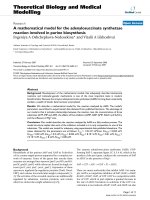
Throughput per hour - % profit
1,200,000

120%

1,000,000

100%

800,000

80%

600,000

60%

400,000

40%

200,000

20%
0%

0

throughput per hour

% unitary profit/unitary total cost

Fig. 1B. Items throughput and profit, ordered in profitability descending trend
The first stage of the optimization indicates the items that contribute to the maximization of the EVA. In
addition, the results of the first model allow analyzing the rest of the portfolio of products taking into
account the references, which reduce less the EVA of the company.


248

Nevertheless, the scenario with the higher value of the objective function activates and chooses the
machines and items the company should produce. These items and machines are used in the stage 2 (lot
sizing). It is very important to analyze the items chosen in this first stage. Commonly the criteria used
for the lot size determination are lower cost, higher throughput and higher unitary profitability (% unitary
profit/unitary total cost). In this work, the proposed objective function couldn´t found any dominance of
these criteria.
Fig. 1A and Fig. 1B show the throughput of products and the profitability for some items respectively.
Fig. 1A shows the items in a descending trend of throughput per hour, while Fig. 1B shows the same
items of Fig. 1A considering unitary profitability (% unitary profit/unitary total cost) ordering them in a
descending trend. This is an important result because shows a different way to select the mix of products
for the company. On Figs. 1A and 1B items included in the armoire product family are highlighted in
red. On Fig. 1A it can be observed that the armoires with the higher throughput are AM6, AM7 and

AM1. And the armoires with the higher profitability (Fig. 1B) are AM5, AM8 and AM1. Nevertheless
the selected armoires in the product selection are AM6, AM7, and AM8; because these are the products
that contribute in a better way to EVA generation. Similar behavior can be observed among the other
product families.
In particular, we have used the EVA as criterion, which is not commonly used. The EVA considers a
holistic point of view considering costs, productivity and profitability. The constraint that forces the
company not concentrate its production and sales in a few items, also forces to the model to activate
some other wildcard items depending on the variability for each scenario.
Table 1
Results of the proposed stochastic model. Source: Owner

AM6
AM7
AM8
B1
B2
B3
B4
C2
CO3
CT1
CV2
E2
MT1
MT2
MT4
MT6
KB2

Final Inventory

Mean Value (Monthly)
252.16
308.63
205.22
699.04
362.81
708.36
552.89
480.47
578
337.43
87.76
57.73
214.68
312.09
327.71
367.33
661.38

Results of the Proposed Model
Batch Size
Number of batches
Mean Value
(Year)
2179.6
9.84
1863.78
8.56
990.6
7.23

2507.43
4.35
1979.69
5.64
3416.51
3.98
3180.83
4.06
2324.05
2.67
3754.08
4.24
1920.88
3.35
1010.73
4.08
1184.86
11.01
5245.3
5.53
1705.57
7.85
1615.93
2.01
2516.46
5.56
3650.08
4.44

Shortage

Mean (Monthly)
3.75
3.58
18.79
56.77
95.77
238.84
269.75
132.05
348.72
195.05
265.46
91.09
1537.4
57.29
146.96
242.41
264.03

Table 1 shows a summary for the results of the 300 scenarios performed. On this table a comparison
between selected items AM6 and CT1 can be performed. AM6 is scheduled an average of 9.84 times in a
year. On the other hand CT1 is scheduled only 3.35 times per year. This happens because AM6 is a very
important item for EVA generation and additionally it has a high sale price and high unitary cost.
Scheduling this valuable items many times the solver tries to minimize their inventory and shortage cost.
This issue can be noticed also when checking the mean shortage and the mean inventory of the two
references. CT1 is not so important for EVA generation (wildcard item) therefore falling into carrying and

 

D. N. Rodado et al. / International Journal of Industrial Engineering Computations 8 (2017)

249

shortage cost costs in these references is not so critical than falling into these costs with EVA relevant
items such as AM6. The proposed model can be applied both for MTS (make to stock) and MTO (make
to order) systems by manipulating the shortage cost, the carrying cost, and variables such as shortage, final
inventory and warehouse available space. Another important issue is that the maximization of the EVA as
the objective function, allows the decision maker to involve costs, earnings, profits and productivity
together.
6. Concluding remarks and future works
In this study, we propose a Stochastic Mixed Integer Linear Programming Model (SILP) for the product
mixing and lot-sizing problem. The decisions of the stochastic model are defined in two steps by
considering variability of the demand. It is proposed as objective function of the SILP model, the
maximization of EVA, the latter is defined as the economic value added generated by the company. The
solution strategy used for the SILP model solution is known as Sample Average Approximation (SAA).
The results of the application of this methodology show that the proposed approach is an effective
decision support tool of product mix and lot sizing problems by considering the expected economic
contribution of products and variability of the demand. In addition, we have demonstrated that the
methodology SAA provides near-optimal solutions for linear stochastic programming problems with
small sample sizes on production problems. Dynamic aspects of the problem, which help to make
decisions according to the demand seasonality and the variability of the prices, could be considered as
future research work. In addition, decisions of scheduling of products and decisions of space constraints
for working process must be taking into account. Finally, applicability of other methods for solving
stochastic linear optimization models and other real cases such as companies with different production
systems could be considered as extensions of this paper.
References
Absi, N., & Kedad-Sidhoum, S. (2008). The multi-item capacitated lot-sizing problem with setup times
and shortage costs. European Journal of Operational Research, 185(3), 1351-1374.
Ahmed, S., Tawarmalani, M., & Sahinidis, N. V. (2004). A finite branch-and-bound algorithm for twostage stochastic integer programs. Mathematical Programming, 100(2), 355-377.

Alejandro, G. H. J.W Escobar, & Álvaro, F. C. (2013). A Multi-Product Lot-Sizing Model for a
Manufacturing Company. Ingeniería Investigación y Tecnología, 14(3), 413-419.
Azaron, A., Tang, O., & Tavakkoli-Moghaddam, R. (2009). Dynamic lot sizing problem with
continuous-time Markovian production cost. International Journal of Production Economics, 120(2),
607-612.
Escobar J.W. (2012). Rediseño de una red de distribución con variabilidad de demanda usando la
metodología de escenarios. Revista Facultad de Ingeniería UPTC, 21(32), 9-19.
Escobar, J. W. (2009). Modelación y Optimización de diseño de redes de distribución de productos de
consumo masivo con elementos estocásticos. Proceedings of XIV Latin American Summer Workshop
on Operations Research (ELAVIO), El Fuerte, México.
Escobar J.W., Bravo, J.J., & Vidal, C.J. (2012). Optimización de redes de distribución de productos de
consumo masivo en condiciones de riesgo. Proceedings of XXXIII Congreso Nacional de Estadística
e Investigación Operativa (SEIO), Madrid, Spain.
Escobar, J. W., Bravo, J. J., & Vidal, C. J. (2013). Optimización de una red de distribución con
parámetros estocásticos usando la metodología de aproximación por promedios muéstrales. Ingeniería
y Desarrollo, 31(1), 135 –160.
Fleischmann, B. (1990). The discrete lot-sizing and scheduling problem. European Journal of
Operational Research, 44(3), 337-348.
Haksever, C., & Moussourakis, J. (2008). Determining order quantities in multi-product inventory
systems subject to multiple constraints and incremental discounts. European Journal of Operational
Research, 184(3), 930-945.


250

Karimi, B., Ghomi, S. F., & Wilson, J. M. (2003). The capacitated lot-sizing problem: a review of models
and algorithms. Omega, 31(5), 365-378.
Kleywegt, A. J., Shapiro, A., & Homem-de-Mello, T. (2002). The sample average approximation method
for stochastic discrete optimization. SIAM Journal on Optimization, 12(2), 479-502.
Lin, C. H. E. N., & QIAO, Z. L. (2010). What influence the Company’s Economic Value Added?

Empirical Evidence from China's Securities Market. Management Science and Engineering, 2(1), 6776.
Mabin, V. J., & Gibson, J. (1998). Synergies from spreadsheet LP used with the theory of constraints—
a case study. Journal of the Operational Research Society, 49(9), 918-927.
Mafla I., Escobar J.W., (2015). Rediseño de una red de distribución para un grupo de empresas que
pertenecen a un holding multinacional considerando variabilidad de la demanda. Revista de la
Facultad de Ingeniería U.C.V., 30(1), 37 – 48.
Marshall, A. (1890). Principles of Political Economy. Maxmillan, New York.
Niebles-Atencio, F. N., & Niera-Rodado, D. N. (2016). A Sule´s method initiated genetic algorithm for
solving QAP formulation in facility layout design: A real world application. Journal of Theoretical
and Applied Information Technology, 84(2), 157.
Paz, J. C., Orozco, J. A., Salinas, J. M., Buriticá, N. C., & Escobar, J. W. (2015). Redesign of a supply
network by considering stochastic demand. International Journal of Industrial Engineering
Computations, 6(4), 521 – 538.
Ray, R. (2001). Economic value added: Theory, evidence, a missing link. Review of Business, 22(1/2),
66.
Rizk, N., & Alain, M. (2001). Supply chain flow planning methods: a review of the lot-sizing literature.
Canada: Universite Laval Canada and Centor. Centre de recherche sur les technologies de
l’organisation réseau (CENTOR)
Rizk, N., Martel, A., & Ramudhin, A. (2006). A Lagrangean relaxation algorithm for multi-item lotsizing problems with joint piecewise linear resource costs. International Journal of Production
Economics, 102(2), 344-357.
Santoso, T., Ahmed, S., Goetschalckx, M., & Shapiro, A. (2005). A stochastic programming approach
for supply chain network design under uncertainty. European Journal of Operational Research,
167(1), 96-115.
Singh, T., & Mehta, S. (2012). EVA VS Traditional Accounting Measures: A Pre-Recession Case Study
of Selected IT Companies. International Journal of Marketing and Technology, 2(6), 95-120.
Su, C. T., & Wong, J. T. (2008). Design of a replenishment system for a stochastic dynamic
production/forecast lot-sizing problem under bullwhip effect. Expert Systems with Applications,
34(1), 173-180.
Van Eijs, M. J. G., Heuts, R. M. J., & Kleijnen, J. P. C. (1992). Analysis and comparison of two strategies
for multi-item inventory systems with joint replenishment costs. European Journal of Operational

Research, 59(3), 405-412.
Van Hoesel, S., Kuik, R., Salomon, M., & Van Wassenhove, L. N. (1994). The single-item discrete lot
sizing and scheduling problem: optimization by linear and dynamic programming. Discrete Applied
Mathematics, 48(3), 289-303.
© 2016 by the authors; licensee Growing Science, Canada. This is an open access article
distributed under the terms and conditions of the Creative Commons Attribution (CCBY) license ( />