Strategic production modeling for defective items with imperfect inspection process, rework, and sales return under two-level trade credit
Bạn đang xem bản rút gọn của tài liệu. Xem và tải ngay bản đầy đủ của tài liệu tại đây (692.82 KB, 34 trang )
International Journal of Industrial Engineering Computations 8 (2017) 85–118
Contents lists available at GrowingScience
International Journal of Industrial Engineering Computations
homepage: www.GrowingScience.com/ijiec
Strategic production modeling for defective items with imperfect inspection process,
rework, and sales return under two-level trade credit
Aditi Khanna, Aakanksha Kishore and Chandra K. Jaggi*
Department of Operational Research, Faculty of Mathematical Sciences, New Academic Block, University of Delhi, Delhi-110 007, India
CHRONICLE
ABSTRACT
Article history:
Received April 4 2016
Received in Revised Format
June 16 2016
Accepted July 8 2016
Available online
July 10 2016
Keywords:
Inventory
Production
Imperfect items
Inspection
Reworking
Two-stage trade credit
Quality decisions are one of the major decisions in inventory management. It affects customer’s
demand, loyalty and customer satisfaction and also inventory costs. Every manufacturing
process is inherent to have some chance causes of variation which may lead to some defectives
in the lot. So, in order to cater the customers with faultless products, an inspection process is
inevitable, which may also be prone to errors. Thus for an operations manager, maintaining the
quality of the lot and the screening process becomes a challenging task, when his objective is to
determine the optimal order quantity for the inventory system. Besides these operational tasks,
the goal is also to increase the customer base which eventually leads to higher profits. So, as a
promotional tool, trade credit is being offered by both the retailer and supplier to their respective
customers to encourage more frequent and higher volume purchases. Thus taking into account
of these facts, a strategic production model is formulated here to study the combined effects of
imperfect quality items, faulty inspection process, rework process, sales return under two level
trade credit. The present study is a general framework for many articles and classical EPQ model.
An analytical method is employed which jointly optimizes the retailer’s credit period and order
quantity, so as to maximize the expected total profit per unit time. To study the behavior and
application of the model, a numerical example has been cited and a comprehensive sensitivity
analysis has been performed. The model can be widely applicable in manufacturing industries
like textile, footwear, plastics, electronics, furniture etc.
© 2017 Growing Science Ltd. All rights reserved
1. Introduction
Quality revolves around the concept of meeting or exceeding customer expectation applied to the product
and service. Achieving high quality is an ever changing, or continuous process, therefore management is
constantly working to improvise quality, so as to serve their customers with good quality products. So,
it becomes inevitable to reduce or remove the defects by screening the complete lot before sale. In view
of this, researchers have lately shown efforts to develop EOQ and EPQ model for the imperfect quality
items. However, the beginning of research on EPQ can be dated back a century ago and was projected
by Taft (1918). Porteus (1986), Rosenblatt and Lee (1986), Lee (1987), Schwaller (1988), Zhang and
* Corresponding author. Tel. Fax.: +91-11-27666672
E-mail: (C. K. Jaggi)
© 2017 Growing Science Ltd. All rights reserved.
doi: 10.5267/j.ijiec.2016.7.001
86
Gherchak (1990) were the first few researchers to study the effect of imperfect quality items on EOQ and
EPQ models. Furthermore, Salameh and Jaber (2000) carried the research by considering that the whole
lot contains a random percentage of defective items with known p.d.f. They also assumed that whole lot
goes through 100% screening process and the sorted out defective items are sold as a single batch at a
discounted price. Later, Sana (2010) examined the production in imperfect quality scenario in which the
production shifts from “in control” to “out of control” state.
It is again impractical to assume that the inspection process is also perfect. Due to certain human errors,
the inspection process leads to errors namely Type-I and Type-II. Due to Type-I error, non-defective
items are classified as defective and due to Type-II error, defective items are classified as non-defective.
This not only leads to customer dissatisfaction but also sales return bringing inconvenience and
frustration to the customers. For the compensation of monetary losses, all the defective items instead of
simply discarding can be reworked after inspection process and again treated as perfect items. This has
invited many researchers to study the EPQ model extensively under real life situations. Raouf et al.
(1983) were among the initial researchers to have inspection errors as a feature in their study. Duffua and
Khan (2005) suggested inspection plans for the mistakes committed by the inspector. Papachristos and
Konstantaras (2006) emphasized on the issue of non-shortages in inventory models with imperfect
quality. Referring to the models of Salameh and Jaber (2000), they pointed out that the conditions
proposed as sufficient ones to guarantee that shortages will not occur and cannot really ensure it. Yoo et
al. (2009) extended the research by adding defect sales and two disposition methods in their formulation.
Khan and Jaber (2011) took similar approach as that of Salameh and Jaber (2000), to reach optimal
solution in imperfect quality environment. One of the earliest researchers in production models who
considered rework processes was Schrady (1967). Hayek and Salameh (2001) threw light on effect of
defective items produced on finite production model. Chiu (2003) developed EPQ model with the
assumption that not all of the defectives are repairable and a proportion goes to scrap and will not be
reworked. A similar model considering service level constraints with rework was developed by Chiu et
al. (2007). Lately, Liu et al. (2009) analyzed the number of production and rework setups used in one
cycle; as well as their sequence and optimal production quantity in each setup. Cardenas-Barron (2009)
also developed an EPQ model with rework by using a planned backorder. Recently, Chung (2011)
revisited the work of Cardenas-Barron to develop a necessary and sufficient condition for the optimal
solution. Yoo et al. (2012) developed imperfect-quality inventory models for various inspection options
i.e. sampling inspection, entire lot screening and no inspection, under one-time improvement investment
in production and inspection reliability. Recently, Wee and Widyadana (2013) studied human errors in
inspection and showed the significance of rework and preventive maintenance on optimal time. Further
Sarkar et al. (2014) revisited the EPQ model with rework process at a single stage manufacturing system
with planned backorders, providing a closed form solution of three different inventory models with three
different distribution density functions. Jaggi et al. (2015) explored the effect of deterioration on two
warehouse inventory model in imperfect quality scenario. Very recently, Jaggi et al. (2016) have
performed elaborated work on imperfect production, inspection and rework process altogether. The
authors have developed a mathematical model with the incorporation of five random variables along with
the condition of shortages.
Furthermore, in order to survive in this set-up of imperfect productions, many businesses lend loan
without interest to their customers as a promotional strategy to increase profitability. Now owing to this
trade credit policy, the suppliers do not require to be paid immediately and may agree a delay in payment
for goods and services already delivered. Until the expiration of the credit period, the creditors can
generate revenue by selling off the items bought on credit and investing the sum in an interest bearing
account. Interest is charged if the account is not settled by the end of credit period. In view of this, Haley
and Higgins (1973) were the first to consider economic order quantity under permissible delay in
payment. Goyal (1985) considered a similar problem including different interest rates before and after
the expiration of credit periods. Aggarwal and Jaggi (1995) extended Goyal’s model by considering
exponential deterioration rate under trade credit. Kim et al. (1995) examined the effect of credit period
A. Khanna et al. / International Journal of Industrial Engineering Computations 8 (2017)
87
to increase wholesaler’s profits with demand as a function of price. Jamal et al. (1997) also generalized
Goyal’s model to allow for shortages. Teng (2002) further analyzed Goyal’s model to include that it is
more profitable to order less quantity and make use for permissible delay more frequently.
In today’s competition–driven world, with the purpose of increasing profit, the retailer also gives some
permissible delay in payment to his own customers. When both supplier and retailer offer credit period
to their respective customers, it is termed as two stage trade credit. This not only indicates the seller's
faith in the buyer, but also reflects buyer's power to purchase now without immediate payment.
Researchers have lately shown efforts in developing two stage trade credit policies. Jaggi et al. (2008)
formulated an EOQ model under two-level trade credit policy with credit linked demand. Ho et al. (2008),
Teng and Chang (2009) also gave replenishment decisions under two stage trade credits. Thangam and
Uthayakumar (2009) extended Jaggi et al. (2008) for perishable items when demand depends on both
selling price and credit period under two-level trade credit policy. Recently, Kreng and Tan (2011)
developed a production model for a lot size inventory system with finite production rate and defective
items which involve imperfect quality and scrap items under the condition of two-level trade credit
policy. Recently, Chung and Liao (2011) gave the simplified solution algorithm for an integrated
supplier–buyer inventory model with two-part trade credit in a supply chain system. Ouyang and Chang
(2013) together explored the effects of the reworking of imperfect quality items and trade credit on the
EPQ model with imperfect product processes and complete backlogging. In this direction, Voros (2013)
worked on the production modeling without the constraint of defective items in the model. The paper
deals with a version of the economic order and production quantity models when the fraction of defective
items is probability variable that either may vary from cycle to cycle, or remains the same as it was in
the first period. Another contribution in this field was given by Hsu and Hsu (2013a) who developed an
economic order quantity model with imperfect quality items, inspection errors, shortage backordering,
and sales returns. A closed form solution is obtained for the optimal order size, the maximum shortage
level, and the optimal order/reorder point. He further investigated the scenario in Hsu and Hsu (2013b)
model where they study two EPQ models with imperfect production processes and inspection errors. The
model focuses on the time factor of when to sell the defective items has a significant impact on the
optimal production lot size and the backorder quantity. The results show that if customers are willing to
wait for the next production when a shortage occurs, it is profitable for the company to have planned
backorders although it incurs a penalty cost for the delay. Very lately, Zhou et al. (2015) considered the
combined effect of trade credit, shortage, imperfect quality and inspection errors to establish a synergic
economic order quantity model, however, they considered one level trade credit with constant demand
and without considering reworking of salvage items. In recent times, Tiwari et al. (2016) discussed the
impact of trade credit and inflation on retailer’s ordering policies for non-instantaneous deteriorating
items in a two-warehouse environment. Same year, Chang et al. (2016) developed a model to study the
impact of inspection errors and trade credits on the economic order quantity model for items with
imperfect quality.
The formal structure of the present model involves imperfect production process, inspection errors, two
disposition methods, two way trade credits and a production model. A strategic production model has
been developed where the supplier supplies the raw material in semi-finished state to the manufacturer
to procure the items and sell them as finished products to his customers i.e. the retailers. Trade credit
policies are used by both i.e. the supplier and the manufacturer for their respective customers as it acts
as a promotional tool for their businesses. Another valid assumption considered here is that of no
shortages. The proposed model jointly optimizes the retailer’s credit period and the lot size by
maximizing expected total profit per unit time. A numerical example is provided to demonstrate the
applicability of the model and a comprehensive sensitivity analysis also has been conducted to observe
the effects of key model parameters on the optimal replenishment policy. The literature has also been
presented in tabular form for better comparison of past papers with the present model.
88
Table 1
Literature Review
Papers
Scrady (1967)
Raouf et al. (1983)
Salameh and Jaber (2000)
Duffua and Khan (2005)
Kim et al. (2009)
Khan and Jaber (2011)
Hayek and Salameh (2001)
Chiu (2003)
Chiu (2007)
Liu et al. (2009)
Chiu (2010)
Kim et al. (2012)
Wee (2013)
Sarkar et al. (2014)
Jaggi et al. (2008)
Voros (2013)
Hsu (2013a)
Zhou et al. (2015)
Yoo et al. (2009)
Jaggi et al. (2016)
This paper
Imperfect
Items
Screening
Process
Screening
Errors
Rework
Sales Return
Trade Credit
Policy
Shortages
Yes
Yes
Yes
Yes
Yes
Yes
Yes
Yes
Yes
Yes
Yes
Yes
Yes
Yes
Yes
Yes
Yes
Yes
Yes
Yes
Yes
No
Yes
Yes
Yes
No
Yes
Yes
Yes
Yes
Yes
Yes
Yes
Yes
Yes
Yes
No
Yes
No
Yes
No
Yes
No
Yes
No
No
No
No
No
No
No
No
No
No
Yes
Yes
No
No
No
Yes
No
Yes
Yes
Yes
Yes
Yes
No
Yes
Yes
No
No
No
Yes
Yes
Yes
Yes
Yes
Yes
Yes
Yes
No
Yes
Yes
Yes
No
No
No
No
No
Yes
No
No
No
No
No
No
No
No
No
No
Yes
Yes
Yes
Yes
Yes
No
No
No
No
No
No
No
No
No
No
No
No
No
No
Yes
No
No
Yes
No
No
Yes
No
No
No
No
No
No
Yes
Yes
Yes
No
Yes
No
Yes
Yes
Yes
Yes
Yes
No
No
No
No
2. Assumptions and Notations
The mathematical model proposed in this paper is based on following assumptions and notations.
1. Demand is a function of retailer’s credit period (N). it can be derived as a differential difference
equation:
D(N+1)-D(N)= R[U- D(N)]
Where
D= D(N)=demand as a function of N per unit time
U= maximum demand
R= rate of saturation of demand (which can be estimated using the past data)
Keeping other attributes like price, quantity, etc. at constant level and by using initial
condition: At N=0, D(N)=u (initial demand), the above differential equation can be
solved as:
1
1
1
i. e.
(1)
1
2.
3.
4.
5.
Time horizon is infinite and insignificant lead time.
Production and Inspection processes are not perfect.
Screening rate is assumed to be greater than the demand rate so as to avoid stock out conditions.
The supplier provides a credit period (M) to the manufacturer, who in turn gives a credit period
(N) to the retailer.
6. All the defect returns are received by the end of production process and then sent for rework.
7. In the model, the defect proportion, proportion of Type-I error, proportion of Type-II error can
be estimated from the past data. Here, these are assumed to follow Uniform distribution.
Parameters
P
λ
P1
Production rate in units per unit time
Production rate of imperfect items(=d*P) in units per unit time
Rework rate in units per unit time
A. Khanna et al. / International Journal of Industrial Engineering Computations 8 (2017)
Production and inspection time
Rework Run time
Cycle length
Remaining time in the cycle i.e. (T-t1-t2)
Proportion of imperfect items
Proportion of non-defective items
Proportion of Type-I imperfection error
Proportion of Type-II imperfection error
Proportion of items sent for rework
Expected value operator
Expected value of α
Manufacturer’s credit period offered by the supplier to settle his accounts (time unit)
Set-up cost for each production run
Production cost per item ($/ item)
Inspection cost per item ($/ item)
Cost of committing Type-I error ($/ item)
Cost of committing Type-II error ($/ item)
Selling price ($/ item)
Salvage cost (< s) ($/ item)
Holding cost per unit item per unit time
Holding cost for each imperfect quality item being reworked per unit time
The max on-hand inventory in units, when the regular process ends
The max on-hand inventory in units, when the rework process ends
Interest earning rate per dollar per unit time per year by the manufacturer
Interest payable rate per dollar per unit in stock per year by the manufacturer
t1
t2
T
t3
d
1-d
q1
q2
r
E(.)
E(α)
M
K
c
i
Cr
Ca
s
v
h
h1
z1
z
Ie
Ip
Decision variables
N
y
Functions
f(d)
f(q1)
f(q2)
f(r)
D(N)
T.R.
T.C.
T.P. i
Zi(y,N)
E
89
,
Optimal values
D*(N)
T*
N*
y*
Z*(y,N)
E[Z*(y,N)]
Retailer’s credit period offered by the manufacturer to settle his account (time unit)
Production lot size for each cycle (in units)
p.d.f. of defective items
p.d.f. of Type-I error
p.d.f. of Type-II error
p.d.f. of items sent for rework
Demand rate, a function of retailer’s credit period in units per unit time
Manufacturer’s Total revenue
Manufacturer’s Total cost
Manufacturer’s Total profit for i=1,2,3,4,5 cases
Manufacturer’s total profit per unit time which is a function of two variables;
y and N for i=1,2,3,4,5 cases
Manufacturer’s Expected Total profit per unit time for i=1,2,3,4,5 cases
Optimal Demand rate for optimal N per unit time
Optimal cycle length
Optimal credit period for the retailer
Optimal production quantity per cycle
Manufacturer’s optimal total profit per unit time
Manufacturer’s optimal expected total profit per unit time
90
3. Model Description and Formulation
When the items are produced within the firm and not purchased from outside to meet the demands, such
a process is known as manufacturing process and the goal of most manufacturing firms is to maximize
the profit by producing the optimal quantity so that there is no overstocking or under stocking. In a 3 tier
supply chain for the production model, the supplier provides raw material to the manufacturer who
processes the semi- finished products to procure the finished item ready for selling to his customers i.e.
the retailers here. The mathematical model used to assist such firms in maximizing the profit by
determining optimal production lot size is called Economic Production Quality (EPQ) model. The
production and inspection rate have to be greater than the demand rate for smooth functioning of the
system and to avoid shortage conditions, respectively, so it is also called Finite Production model. In any
production process due to certain reasons like deterioration, improper transport, weak process control or
any other factor, the production may shift to imperfect production process in which not all the items are
of good quality. Due to this whole lot goes through the inspection process which is also prone to errors,
i.e. Type-I which causes direct loss to the manufacturer by stopping him to generate revenue on full sales
since it identifies a perfect item as defective and Type-II inspection error which not only causes monetary
losses but also customer dissatisfaction which is more difficult to recover. Due to this error, a defective
item is identified as non-defective, thereby passing on to customers and resulting in defect sales return.
Production and inspection occur simultaneously. After the end of production process, rework of defective
item begins. Not all defective items are sent for rework; some are discarded and sold as scrap. Demand
is continuously satisfied from perfect or reworked items. In this paper, a three tier supply chain has been
considered, where production and inspection process is not perfect.
In producing lot y, due to imperfect production quality, d proportion of defective items are produced with
known probability density function f(d). So, lot y has defective items as dy and non-defective items as
(1-d)y. Due to imperfect inspection process, there is generation of Type-I and Type-II errors, given their
respective proportions of q1=Pr (items screened as defects | non- defective items) and q2=Pr (items not
screened as defects | defective items) (0
are determined inter-dependently by q1, q2, and y. In Type-II error, non-defective items are falsely treated
as defects thereby losing an opportunity to make more profit by selling them to customers at selling price
(s). Due to Type-I error, (1-d)q1y units among the non-defective items of (1-d)y are falsely treated as
defects, leaving (1-r)(1-q1)y units of the non-defects as perfect and ready for sale. In Type-II error, the
defective items are wrongly sold to the customers by treating them like perfect or non-defective items,
resulting in sales return and loss of goodwill. Due to Type-II error, dq2y units among the defective items
of dy are falsely treated as non-defects, leaving d(1-q2)y units among the defects. Since demand D(N) is
satisfied by perfect items only, it becomes practically important to examine imperfect production and
inspection process which affects a firm’s profitability. After the inspection of the entire lot y, all the
sorted-out non-defective items are summed as [dq2y+(1-d)(1-q1)y] which include falsely inspected
defects (Type-II error) and successfully inspected non-defects respectively and the total sorted out
defective items are summed up as [d(1-q2)y + q1(1-d)y] which include successfully inspected defects and
falsely inspected non-defects (Type-I error) respectively. Those falsely inspected defects (dq2y) result in
sales return when passed on to customers due to quality dissatisfaction. Two disposition methods are
employed to settle out defective items and defect returns. One is rework process and other is discarding
them as scrap. The defect returns are assumed to re-enter the inventory cycle continuously like demand
and get accumulated over the length of period T so that the defect returns and defective items can be sent
for rework together at a constant rate P1 in the next cycle after time duration t1. Not all the defective items
go for the rework process, some are discarded beforehand at a lesser price v (
respectively. So, the reworked items are [d + (1-d)q1]ry and salvaged items are [d+(1-d)q1](1-r)y.
Reworked items are treated as good as perfect items and sold at the same selling price (s). Disposing off
A. Khanna et al. / International Journal of Industrial Engineering Computations 8 (2017)
91
of salvage items occurs at the end of each production and inspection cycle as in Salameh and Jaber
(2000).
Lot y
Inspection of lot y
dy
(1-d)y
Defective
Classification as
Def. item (1-q2)
Non-Defective
Classification as
Classification as
Non. Def item (q2) Def. item (q1)
d(1-q2)y
dq2y
q1(1- d) y
Classification as
Non.Def(1-q1)
(1-d)(1-q1) y
Defect Returns
Sales
Salvage [d+q1 (1- d)](1-r)y
d(1-q2) y + dq2y + q1 (1-d)y
= d y + q1(1- d) y
= [d+ q1 (1- d)] y
(For disposal)
[d+q1 (1-d)]ry
Rework
Fig. 1. Flowchart of the processes taking place
It is also assumed that there is a delay in payment allowed up to a credit limit and there is no interest
charged within this limit. However if the account is not settled within this limit, there is interest charged
beyond the credit point. When both supplier and retailer offer credit period to their respective customers,
this is termed as two stage credit policy which has been considered in this paper. Demand is taken as a
function of customer’s credit period N and supplier’s credit period is M. Here, N is taken as the second
decision variable and has been jointly optimized with y. Finally, no shortages are allowed in each cycle
T. The sequence of all the above described events is shown in Fig. 1. The behavior of the inventory model
describing the whole scenario is shown in Fig. 2. The aim of this model is to determine the optimal
production lot size y and the retailer’s credit period N that maximizes the expected total profit per unit
time (E[Z(y,N)]). Various factors contributing to the total profit per unit time (T.P.U.) are: Total Revenue,
Total Cost, Interest Earned and Interest Paid.
92
(a) Inventory
Level
y
P
Defective Items
P‐λ
z
P1‐D
z1
P‐D‐λ
A1
A2
A3
t2
t 1
t3
Time
T
(b)
Inventory
Level
Returned
Items
dq2y
A5
t 1
(c) Inventory level
t1
Time
(d) Inventory level
P1
Defective Items
[ d(1-q2) + q1(1-d) ] y
A 4
t 1
T
Time
Rework Items
[d+q1 (1-d)]ry
A6
t1
t 2
Time
Fig. 2. Inventory behavior of (a) imperfect production and inspection system, (b) defect returns, (c)
defective items sorted through inspection process, (d) reworked items
The conditions which conform that there will be no shortage conditions in the model are:
a. Total number of perfect items should be greater than the demand during the inspection period i.e.
1
1
, i.e.
(2)
A. Khanna et al. / International Journal of Industrial Engineering Computations 8 (2017)
93
where
1
1
(3)
β being a combination of random variables viz. d, q1, q2, is also a random variable.
So,
E[β] = E[dq2] + (1-E[d]) (1-E[q1])
(3.1)
b. Total number of perfect items(including reworked items) after the inspection process should be
greater than the demand during rest of the period i.e.
1
1
1
i.e.
(4)
where
1
(5)
δ being a combination of random variables viz. d, q1, is also a random variable.
So,
E[δ] = E[d] + E[q1] (1-E[d])
(3.2)
From Fig. 2, some basic formulae are derived:
λ
Also,
(6)
(7)
(8)
Using Eq. (6), (7), the values of z, z1 are derived:
(9)
(10)
Therefore, from Eq. (6), (7), (8) and (10)
Cycle length
Σ , i = 1, 2, 3 i.e.
(11)
Also, by following the same procedure as that of Yoo et al. (2009), the cycle length can be obtained from
the depletion time of all the serviceable items sold as per demand rate, i.e
94
from Eq. (3.1) and (3.2)
(12)
where
, say
(13)
α being a combination of random variables viz. β, δ, r is also a random variable.
So,
E[α] = E[β] + E [δr]
(3.3)
Various components of total revenue are:
i.
Sales revenue of Non-Defective items =
ii.
Revenue loss from Defect Refund =
iii.
Sales revenue of Reworked Items =
iv.
Sales revenue of Salvage Items =
1
1
(14a)
(14b)
1
(14c)
1
1
(14d)
By using Eqs. (14a-14d), we obtain:
Total Revenue (T.R.) = Sales revenue of Non-Defective items – Revenue loss from Defect
Refund + Sales revenue of Reworked Items + Sales revenue of Salvage Items
1
1
(T.R.)
1
1
1
1
(15)
Various components of cost function are:
i. Setup Cost =K
ii. Purchase Cost =
iii. Inspection Cost =
iv. Cost of committing Type-I error =
v. Cost of committing Type-II error =
vi. Rework Cost =
1
vii. Inventory Holding Cost =
1
By using Eqs. (16a-16g), we obtain:
(16a)
(16b)
(16c)
(16d)
(16e)
(16f)
1
1
(16g)
1
Total Cost (T.C.) = Setup Cost + Purchase Cost + Inspection Cost + Cost of committing Type-I error +
Cost of committing Type-II error + Rework Cost + Inventory Holding Cost
. .
(17)
1
1
1
1
1
A. Khanna et al. / International Journal of Industrial Engineering Computations 8 (2017)
95
Now, depending upon the value of M, N and T, the value of interest earned and interest paid is calculated
for five distinct possible cases Zj(y,N); j=1, 2, 3, 4, 5 viz.
Case (i) N ≤ M ≤ t1+N ≤ T+N
Case (ii) N ≤ t1+N ≤ M ≤ T+N
Case (iii) N ≤ t1+ t2+N ≤ M ≤ T+N
Case (iv) T+N≤ M
Case (v) M ≤ N ≤ T+N
Case i
N ≤ M ≤ t1+N ≤ T+N
From the Fig. 3, it is clearly visible that the interest earning period for the manufacturer is from N to M,
as he starts getting his actual sales from N. At M, the manufacturer settles his account with the supplier
and arranges for the finances to make the payment to the supplier for the left over stock which are the
remaining perfect and reworked items used to satisfy demand and the items for disposal, which include
the actual defectives, sales return and falsely sorted defectives. Interest is charged on the unsold items
for the time M to T+N.
Revenue
Interest
Paid
Interest
Earned
N
M
t1+N
t1+ t2+N
T+N
Time
Fig. 3. N ≤ M ≤ t1+N ≤ T+N
(18)
Interest Earned (Ie1)
Interest Payable (Ip1)
1
1
(19)
(Ip1)
1
Total Profit (T.P.1) = Total Revenue (T.R.) – Total Cost (T.C.) + Interest Earned (Ie1) – Interest
Payable (Ip1)
(20)
1
1
(T.P.1)
1
1
96
1
By using Eq. (12) and Eq. (20), we get:
1
1
. . .
E
(21)
2
1
1
1
By using Renewal- reward theorem, we get:
Expected Total Profit per unit time (E
,
(22)
)
where, E[.] denotes the expected value.
Case ii
N ≤ t1+N ≤ M ≤ T+N
Revenue
Interest
Paid
Interest
Earned
M
N
t1+N
t1+ t2+N
T+N
Time
Fig. 4. N ≤ t1+N ≤ M ≤ T+N
As visible in Fig. 4, the manufacturer earns interest on sales revenue from N to M, as he gets his first
delivery of cash at N. These items include the defect returns from the market for the time period (
A. Khanna et al. / International Journal of Industrial Engineering Computations 8 (2017)
97
, ). Since the items for disposal have also been sold at t1, he earns additional interest on these items
also. The whole amount is accumulated in an interest bearing account till the time M. After the settlement
of manufacturer’s account with the supplier at M, the unsold items have to be financed by the
manufacturer on his own to make the payment to the supplier which constitutes the remaining perfect
items, reworked items used to satisfy the demand.
+
Interest Earned (Ie2)
1
1
1
(Ie2)
(23)
Interest Payable (Ip2) =
(24)
(Ip2)
Total Profit (T.P.2) = Total Revenue (T.R.) – Total Cost (T.C.) + Interest Earned (Ie2) – Interest
Payable (Ip2)
. .
1
1
1
1
(25)
1
By using Eq. (12) and Eq. (25), we get:
E
1
. . .
2
1
By using Renewal- reward theorem, we get:
1
1
1
26
98
Expected Total Profit per unit time (E
,
(27)
)
–
where E[.] denotes the expected value.
Case iii
N ≤ t1+t2+N ≤ M ≤ T+N
This is the case where the manufacturer earns revenue by selling the items up to M, beginning from time
N. These items include the perfect items along with a proportion of reworked items and also the items
disposed as scrap at t1. He arranges for the finances to pay to the supplier for the unsold inventory lying
in the period (t1 +t2+N, T+N) at some specified rate of interest as depicted in Fig. 5.
Interest
Paid
Revenue
Interest
Earned
M
N
T+N
t1+ t2+N
t1+N
Time
Fig. 5. N ≤ t1+t2+N ≤ M ≤ T+N
Interest Earned (Ie3) =
1
1
(28)
1
Interest Payable (Ip3) =
(29)
Total Profit (T.P.3) = Total Revenue (T.R.) – Total Cost (T.C.) + Interest Earned (Ie3) – Interest
Payable (Ip3)
A. Khanna et al. / International Journal of Industrial Engineering Computations 8 (2017)
. .
1
99
(30)
1
1
1
1
By using Eq. (12) and Eq. (30), we get:
1
. . .
(31)
1
E
2
1
1
1
By using Renewal- reward theorem, we get:
Expected Total Profit per unit time (E
,
)
(32)
–
where E[.] denotes the expected value.
Case iv
T+N ≤ M
As explains the Fig. 6, this is the case of larger interest period resulting in no interest paid by the
manufacturer to the supplier. He not only earns interest on the sales revenue generated by the selling of
perfect and reworked items as per demand from time N to T but also an additional interest from the sale
of defective lot for the time period (t1, M) and on the whole lot for the time period (T, M).
100
Revenue
Interest
Earned
N
t1+N
t1+ t2+N
M
T+N
Time
Fig. 6. T+N≤ M
Interest Earned (Ie4) = s
1
1
(Ie4)=
(33)
1
Interest Payable (Ip4) = 0
(34)
Total Profit (T.P.4) = Total Revenue (T.R.) – Total Cost (T.C.) + Interest Earned (Ie4) – Interest
Payable (Ip4)
. .
1
(35)
1
1
1
1
By using Eq. (12) and Eq. (35), we get:
E
1
. . .
1
2
(36)
1
1
1
A. Khanna et al. / International Journal of Industrial Engineering Computations 8 (2017)
101
By using Renewal- reward theorem, we get:
,
Expected Total Profit per unit time (E
(37)
)
–
where E[.] denotes the expected value.
Case v
M ≤ N ≤ T+N
Revenue
Interest
Paid
M
N
t1+N
t1+ t2+N
T+N
Time
Fig. 7. M ≤N≤ T+N
As shown in Fig. 7, this is the case of smallest credit period where all the units are financed by the
manufacturer from his own pocket, ensuring zero interest earned, to settle his account with the supplier.
This is because the manufacturer gets his first payment at N, which happens to be after the expiration of
his credit period i.e. M.
Interest Earned (Ie5)
Interest
Payable
0
(Ip5)
(38)
1
1
(Ip5)
(39)
1
Total Profit (T.P.5) = Total Revenue (T.R.) – Total Cost (T.C.) + Interest Earned (Ie5) – Interest
Payable (Ip5)
102
. .
(40)
1
1
1
1
1
By using Eq. (12) and Eq. (40), we get:
1
. . .
E
(41)
1
2
1
1
1
By using Renewal- reward theorem, we get:
Expected Total Profit per unit time (E
,
(42)
)
–
–
Hence, the manufacturer’s total profit per unit time is:
,
,
,
,
,
,
if
if
if
if
if
A. Khanna et al. / International Journal of Industrial Engineering Computations 8 (2017)
103
4. Optimal Solution
In this model, the profit function, Z(y,N), is a function of two decision variables out of which one is
discrete, i.e., N, and other is continuous, i.e., y. In order to find the optimal values of N and y which
jointly maximizes the expected total profit per unit time, the value of N is taken as fixed.
Case wise proof of optimality is shown below.
Case (i) N ≤ M ≤ t1+N ≤ T+N
*
To determine the optimal value of y, say y , which maximizes the function of E
first-order necessary condition of optimality must be satisfied:
,
0 i.e.
First we partially differentiate E
,
,
the following
with respect to y, using Eq. (22).
(43)
,
On setting Eq. (43) equal to zero, we get the optimal production size y* as:
∗
(44)
Further, it may be observed that when d, q1, q2, r are just known values rather than random variables and
when N is fixed, then y* can be computed from:
′
,
0 i.e.
(45)
=0
On setting Eq. (45) equal to zero, we get the optimal production size y* as:
(46)
∗
104
Further, to prove the concavity of the expected profit function, the following second-order sufficient
condition of optimality must hold:
,
By taking second order derivative of E
,
with respect to y, we obtain
,
For satisfying the condition of optimality,
,
(47)
0
; true for fixed value of N also.
i.e.
Case (ii) N ≤ t1+N ≤ M ≤ T+N
To determine the optimal value of y, say y * , which maximizes the function of E
first-order necessary condition of optimality must be satisfied:
,
0i.e.
First we partially differentiate E
,
,
, the following
with respect to y, using Eq. (27).
(48)
,
On setting Eq. (48) equal to zero, we get the optimal production size y* as:
(49)
∗
Further, it may be observed that when d, q1, q2, r are just known values rather than random variables and
when N is fixed, then y* can be computed from:
′
,
0 i. e.
(50)
=0
A. Khanna et al. / International Journal of Industrial Engineering Computations 8 (2017)
105
On setting Eq. (50) equal to zero, we get the optimal production size y* as:
(51)
∗
Further, to prove the concavity of the expected profit function, the following second-order sufficient
condition of optimality must hold:
,
0
By taking second order derivative of E
,
with respect to y, we obtain
,
For satisfying the condition of optimality,
,
0
i.e.
(52)
; true for fixed value of N also
Case (iii) N ≤ t1+t2+N ≤ M ≤ T+N
To determine the optimal value of y, say y * , which maximizes the function of E
first-order necessary condition of optimality must be satisfied:
,
,
, the following
i.e.
First we partially differentiate E
,
with respect to y, using Eq. (32).
(53)
0
On setting Eq. (53) equal to zero, we get the optimal production size y* as:
(54)
∗
Further, it may be observed that when d, q1, q2, r are just known values rather than random variables and
0 i.e.
when N is fixed, then y* can be computed from: ′ ,
106
(55)
=0
On setting Eq. (55) equal to zero, we get the optimal production size y* as:
(56)
∗
Further, to prove the concavity of the expected profit function, the following second-order sufficient
condition of optimality must hold:
,
0
By taking second order derivative of E
,
with respect to y, we obtain
,
For satisfying the condition of optimality,
,
0
i.e.
(57)
; true for fixed value of N also
Case (iv) T+N ≤ M
To determine the optimal value of y, say y * , which maximizes the function of E
first-order necessary condition of optimality must be satisfied:
,
0 i.e.
First we partially differentiate E
,
,
, the following
with respect to y, using Eq. (37).
(58)
=0
On setting Eq. (58) equal to zero, we get the optimal production size y* as:
A. Khanna et al. / International Journal of Industrial Engineering Computations 8 (2017)
107
(59)
∗
Further, it may be observed that when d, q1, q2, r are just known values rather than random variables and
0 i.e.
when N is fixed, then y* can be computed from: ′ ,
(60)
=0
On setting Eq. (60) equal to zero, we get the optimal production size y* as:
(61)
∗
Further, to prove the concavity of the expected profit function, the following second-order sufficient
condition of optimality must hold:
,
0
By taking second order derivative of E
,
with respect to y, we obtain
(62)
,
therefore
,
0 ; true for fixed value of N also.
Case (v) M ≤ N ≤ T+N
To determine the optimal value of y, say y * , which maximizes the function of E
first-order necessary condition of optimality must be satisfied:
,
0i.e.
First we partially differentiate E
,
with respect to y, using Eq. (42).
,
, the following
108
(63)
=0
On setting Eq. (63) equal to zero, we get the optimal production size y* as:
(64)
∗
Further, it may be observed that when d, q1, q2, r are just known values rather than random variables and
0 i.e.
when N is fixed, then y* can be computed from: ′ ,
(65)
=0
On setting Eq. (65) equal to zero, we get the optimal production size y* as:
(66)
∗
Further, to prove the concavity of the expected profit function, the following second-order sufficient
condition of optimality must hold:
,
0
By taking second order derivative of E
,
with respect to y, we obtain
(67)
,
Therefore,
,
0, true for fixed value of N also.
A. Khanna et al. / International Journal of Industrial Engineering Computations 8 (2017)
109
5. Special Cases
To verify the formulation of present model, this section provides a general framework to various
previously published articles.
a) In the existing model, if the formulation is confined to only imperfect quality and inspection errors
but not rework and the production rate is assumed to be infinite, then the model reduces to Jaber et
al (2011) model.
i.e. Setting P → ∞, d 0, q1 0, q2 0, λ = constant, r = 0, M = 0, N = 0, Ie = 0, Ip = 0; this
implies δ = d + q1 (1- d), β = dq2 + (1- d) (1- q1), α = dq2 + (1- d) (1- q1).
Then equations (44), (49), (54), (59), (64) can simplify to:
(69)
∗
1
where
b) Suppose the assumption of imperfect quality is removed from the model but the concept of trade
credit with credit-linked demand function is still applied. Also if the production rate approaches to
infinity, then there is no production of imperfect quality items and hence the model reduces to the
EOQ model of Jaggi et al (2008).
i.e. Setting P → ∞, d = 0, q1 = 0, q2 = 0, r = 0; this implies λ = 0, δ = 0, β =1, α =1.
Then equations (44), (49), (54), (59), (64) can simplify to:
∗
(70)
∗
(71)
∗
(72)
c) The traditional EOQ model with imperfect quality formulated by Salameh and Jaber (2000) can be
derived from this present model by neglecting the assumptions of trade credit and inspection errors
along with rework.
i.e. Setting P → ∞, d 0, q1 = 0, q2 = 0, r = 0, M = 0, N = 0, Ie = 0, Ip = 0; this implies λ = 0, δ
= d, β =1 – d, α = 1 – d.
(73)
∗
d) In the present model, if the assumption of imperfect quality is relaxed and trade credit is also removed
from it, then there will be no rework done and the formulation reduces to that of classical EPQ model.
i.e. Setting d = 0, q1 = 0, q2 = 0, r = 0, M = 0, N = 0, Ie = 0, Ip = 0 ; this implies λ = 0, δ = 0, β
=1, α =1.
Then Eq. (45), Eq. (50), Eq. (55), Eq. (60) and Eq. (65) can simplify to:
∗
(74)