Phân tích dẻo kết cấu khung cột thép dầm liên hợp chịu tải trọng tĩnh tt tiếng anh
Bạn đang xem bản rút gọn của tài liệu. Xem và tải ngay bản đầy đủ của tài liệu tại đây (2.16 MB, 28 trang )
MINISTRY OF EDUCATION AND TRAINING
MINISTRY OF CONSTRUCTION
HANOI ARCHITECTURAL UNIVERSITY
========o O o========
HOANG HIEU NGHIA
PLASTIC ANALYSIS OF THE FRAME WITH STEEL
COLUMN AND COMPOSITE STEEL-CONCRETE
BEAM SUPPORT THE STATIC LOAD
MAJOR: BUILDING AND INDUSTRIAL CONSTRUCTION
CODE: 62 58 02 08
ABSTRACT DOCTORAL THESIS
BUILDING AND INDUSTRIAL CONSTRUCTION
HANOI, 2020
The thesis has been completed at:
Hanoi Architectural University
Scientific instructors:
1. Assoc. Prof. PhD. Vu Quoc Anh
2. Assoc. Prof. PhD. Nghiem Manh Hien
Reviewer 1: Prof. PhD. Nguyễn Tiến Chương
Reviewer 2: PhD. Nguyễn Đại Minh
Reviewer 3: Assoc. Prof. PhD. Nguyễn Hồng Sơn
This thesis is defended at the doctoral thesis review board at the Hanoi Architectural
University.
At …… hour - June ….st, 2020
The thesis can be found at:
1. National Library
2. Library of Hanoi Architectural University.
1
PREAMBLE
1. The urgency of the thesis
In recent years, the research and application and development of steel - concrete composite
structures in the world and in Vietnam in the field of structural construction has been
interested by researchers and engineers.
When analyzing and calculating structures, they often use traditional design methods,
including 2 steps: Step 1: Using linear elastic analysis and the principle of collaboration to
determine internal forces and displacements of structural system. Step 2: Check the bearing
capacity, stress limits, stability of each individual component.
This traditional design method has been applied for a long time and has the advantage of
simplifying the design work of an engineer. However, it does not clearly show the nonlinear
relationship between load and displacement, does not clearly show the nonlinearity of the
structural material, has not fully considered the behavior of the entire structure so it leads to
the material fee. The problem of nonlinear analysis, the force-displacement relationship is
nonlinear, must be repeat solved because the structure has been deformed with the previous
load and the structural stiffness is weakened, the computer will update the geometric data,
material properties after each load change so that it will be close to the actual behavior of the
structure. Recently, in the world, when analyzing nonlinear structures, in the standards and
researchers often use two basic methods: zone plastic method and plastic hinge method.
The zone plastic method considers the development of the plastic zone slowly as the force
exerts on the structure, the plasticity of the elements will be modeled by discrete components
of a finite element (divide element bar into n elements) and divide the section into fibers. This
method is an accurate way to test other analytical methods, but this method is complex and
requires a large analysis time (hundreds of times calculated by the plastic hinge method according to Ziemian). Therefore it is not suitable for calculating the actual building, only
suitable for simple structures, so this method is rarely applied in practice.
The plastic hinge method is a simplified model of the real structure with the assumption
that the length of plastic zone lh = 0, whereby it is assumed that during the process of bearing
plastic deformation appears and develops only at the two ends of the element, the remaining
sections in the bar remain elastic deformation. When conducting plastic analysis, the
researchers used the plastic surfaces of Orbison 1982, AISC-LRFD 1994 to consider the yield
condition of the cross section, the plastic surfaces has many limitations so it has not been
reflected realable behavior of structural systems under load.
Through the above analysis, it can be seen that the problem of constructing the plastic
analysis method of the frame structure with steel column and composite beam support the
static load for the problem of spreading plasticity analysis of the structural system and the
limit load problem of the system the structure, including the spreading plasticity of the
composite beam section, the steel column and the plastic deformation zone along the element
length and the plastic flow rate of the section, is significant scientific and practical in
analyzing the structure and necessary to be researched and applied.
Therefore, the thesis chooses the research topic: "Plastic analysis of the frame structure
with steel column and composite steel-concrete beam support the static load"
2. Research purposees
i) Building the curve (M-) relationship of the composite steel-concrete beam taking into
account the plasticity of the material to reflect the actual behavior of the composite beam
structure support load; ii) Building the equation of elastic limit surface, intermediate plastic
surface, fullly plastic surface (failure surface) of the doubly symmetrical wide flange I-
2
section under axial force combined with biaxial bending moments to predict the bearing
capacity of column section steel and builded plastic surface have been applicated into the
nonlinear analysis of structural systems; iii) Building a finite elements method and computer
program applied to nonlinear analysis of the frame structure with steel column and composite
steel-concrete beam considers the plasticity of the material and the distributed plasticity of
the structural system.
3. Object and scope of researchs
- Object of research: Nonlinear analysis of the frame structure with steel column and
composite steel-concrete beam support static load considers the plasticity of the material
- Scope of research: beam structure, plane frame structure with steel columns and
composite steel-concrete beams; model of steel materials regardless of the consolidation
period and nonlinear model of tensile and compressive concrete materials; plastic analysis
model of the structural system: plastic deformation model spread along the element length;
load applied to the structure: static and non-reversible load during the analysis; regardless of
the effect of shear deformation in the component; not taking into account the local buckling
of the section and the lateral buckling of the component; geometrical nonlinearities are not
considered in the analysis process.
4. Research Method
- Using the theoretical research method (analytic method) to develop the nonlinear
analysis theory of the frame structure with steel column and composite steel-concrete beam
considering the plasticity of the material and the distributed plasticity of the system structure.
- Applying nonlinear decomposition algorithms to build computer programs based on
theoretical research results and use to verify the achieved results, in order to accurately and
ensure reliability, as well as the feasibility of the results achieved.
5. Scientific and practical significance of the thesis
i) Building the curve (M-) relationship of the composite steel-concrete beam taking into
account the plasticity of the material to reflect the actual behavior of the composite steelconcrete beam structure support load; ii) Building the equation of elastic limit surface,
intermediate plastic surface, fullly plastic surface (failure surface) of the doubly symmetrical
wide flange I-section under axial force combined with biaxial bending moments to predict the
bearing capacity of column section steel and builded plastic surface have been applicated into
the nonlinear analysis of structural systems; iii) Building a finite elements method with plastic
multi-point bar elements and computer program applied to nonlinear analysis of the frame
structure with steel column and composite steel-concrete beam considers the plasticity of the
material and the distributed plasticity of the structural system; iv) Building an application
computer program for nonlinear analysis of of the frame structure with steel column and
composite steel-concrete beam considers the plasticity of the material and the distributed
plasticity of the structural system reliably and effectively, apply the program to perform
plastic analysis problems.
6. New contributions of the thesis
a) Building the curve (M-) relationship of the steel and composite steel-concrete beam
to determine the tangent stiffness of these components at different points when the material
works in the elastic phase, elastic - plastic and plastic. Establish SPH program to build this
relationship.
b) Building the equation of elastic limit surface, intermediate plastic surface, fullly plastic
surface (failure surface) of the doubly symmetrical wide flange I-section subjected to axial
force combined with biaxial bending moments to predict the bearing capacity of section steel
column corresponding to a certain design load.
3
c) Building calculations by finite element method and computer program to analysis the
frame structure with steel column and composite steel-concrete beam, taking into account the
material nonlinearity when forming multipurpose plasticity points. From this application
program, it is possible to determine the limit load factor, plastic flow rate of the section,
internal force, displacement of the structure corresponding to different load levels, thereby
determining the amount of security full reserve of the structure compared to the design data.
7. The structure of the thesis
The thesis has 4 chapters, introduction, conclusion and appendices
CONTENTS
CHAPTER 1. OVERVIEW OF RESEARCH ISSUES
1.1. Introduction of the frame structure with steel column and composite steel-concrete
beam
Studies of composite structures in the world are increasingly being studied more and in
many different approaches. In Vietnam, this type of structure has only been studied and
applied in the last 10 years and mainly focuses on the study of components and connection
calculations, the overall analysis of the structure when the load is low researched, so the
approach to studying this type of structure has scientific and practical significance in the
construction industry. Within the scope of the thesis, the author has just stopped at studying
plane frames with steel columns and composite steel-concrete beams.
1.2. Trends in analysis, design of steel structures and composite structures
Currently,when analyzing
and calculating steel structure
and composite structure, it is
often
used
traditional
methods (Figure 1.1). All
three methods of ADS, PD,
LRFD
require
separate
inspection
of
each
component, especially taking
into account the K factor, not
considering the full behavior
of the entire structure so that
Figure 1.1. structural design and analysis method
it leads to waste material.
Therefore, it is necessary to study modern design (advanced analysis) and only perform in
one design step because it will accurately reflect the actual working of the structural system,
accurately predict the type of plastic demolition and the limited load of the frame structure
under static load and is essential to the reliability of the design.
1.3. Nonlinear analysis and nonlinear analysis levels
1.3.1. Nonlinear analysis
The problem of nonlinear analysis, the force-deformation relationship is a curve, so it must
be cyclic solved because the structure has been deformed with the previous load and the
structural stiffness is weakened, the computer will update the geometric data, material
properties after each load change. The two basic methods used by the researchers when
analyzing nonlinear structures are the plastic hinge method and the plastic zone method
(Figure 1.2). Some researches on nonlinear materials such as Chan and Chui, White, Wrong,
Chen and Sohal, Chen, Kim and Choi, Yong et al, Orbison and Guire, Nguyen Van Tu and
Vo Thanh Luong.
4
1.3.2. Nonlinear analysis levels
In structural analysis, it is difficult to model all nonlinear factors related to structural
behavior as in reality in detail. The most common levels of nonlinear analysis are described
by the behavioral curves of the static load frame by authors Chan and Chui, Orbison, Nguyen
Van Tu, Vu Quoc Anh, Nghiem Manh Hien, Balling and Lyon refers to: first-order elastic
analysis, second-order elastic analysis, first-order elastic plastic analysis, second-order elastic
plastic analysis.
1.4. Nonlinear model of steel and concrete materials
The thesis used the ideal elastic model according to Eurocode 3 for steel materials, Kent
and Park models (1973) for compressible concrete materials, Vebo and Ghali models (1977)
for tensile concrete materials.
1.5. Moment – curvature relationship of steel section beam (M-)
The process of plastic flow on the section consists of 3 stages: elastic, elastic-plastic and
fully plastic (Figure 1.3) ASCE, Michael, Vrouwenvelder.
Figure 1.2. Methods of nonlinear material analysis
Figure1.3.(M-)relationship
of section steel beam
1.6. Plastic surface of steel columns
The concept of plastic surface is given to mention the simultaneous effect of axial force
and bending moment based on internal force of element. When the bending moment and the
axial force in the element reach the yield surface, the plastic hinge is formed. Some typical
plastic surface has been proposed and applied with many studies: Orbison, Duan and Chen,
AISC-LRFD. This thesis presents the method of constructing the intermediate plastic surface
to show the plastic spread across the section in the plastic analysis process of the structure.
1.7. The method of the frame structure analysis when plastic hinge formde
The popular analysis method is
the finite element method as
shown in Figure 1.4 with many
authors used to analyze such as:
Chan and Chui, White, Wrong,
Chen, Kim and Choi, Orbison and
et al, Liew and Chen, Kim and
Choi , Cuong and Kim, Doan Ngoc
Tinh Nghiem and Ngo Huu Cuong,
Figure 1.4. beam - column element model in finite
element
Abaqus, Ansys, Midas, Adina.
5
CHAPTER 2: BUILDING MOMENT – CURVATURE RELATIONSHIP OF STEEL
SECTION BEAM AND PLASTIC SURFACE OF STEEL SECTION COLUMN
2.1. Building momnent – curvature relationship of steel section beam by the analytical
method
The building of moment - curvature relationship of beam section to calculate tangent
stiffness at the plastic deformation positions, is the basis for element stiffness and is used in
the plastic analysis problem of the structural frame shown in the following chapters. Survey
deformation stress diagram of section I steel beam as shown in Figure 2.1.
M
M
0
Figure 2.1. Stress and deformation diagram of section I in the main axis z
2.1.1. Plastic moment in main axis (axis z)
- Elastic rotation in axis z: z,e 2f y / hE
- Elastic moment: M z,e 2 z E b w h t bf h h t
2 2
3 2
3
3
3
fy h
b w t bf
3 h 2
- Elastic limit moment: M z 4
3
(2.1)
(2.2)
3
h 3 h
t
2 2
(2.3)
- Elastic-plastic moment:
+ Case
2 fy
hE
z
Eb
Mz 2 z w
3
+ Case z
2 fy
h 2t E
h z Ebf
t
3
2
3
2 fy
h 2t E
or 0 z , p
2 fy
h 2t E
f y h 3 f y b f
t
z E 2
2
or z , p
3
2 fy
h 2t E
2 fy
hE
2 fy
hE
2 fy
2t
E h 2t h
h 2 f y 2
2 z E
(2.4)
2 fy
2t
E h 2t h
f b h 2 f b f 2 f b t
Mz 2 y w t y w y y f h t
6 z E
2
2 2
2
f b
f bt
- Maximum moment value: M z,max 2 y w h t y f h t
2
2 2
(2.5)
(2.6)
2.1.2. Plastic moment in auxiliary axis (axis y)
- Elastic rotation in axis y: y ,e 2 f y / b f E
- Elatic moment: M y 2b3f t b3w h 2t y E /12
(2.9)
(2.10)
- Elastic limit moment: M y,e 2b3f t b3w h 2t f y / 6b f
- Elastic-plastic moment:+ Case
2 fy
bf E
y
2 fy
bw E
or 0 y , p
(2.11)
2 fy
bw E
2 fy
bf E
2 f y b f bw
E bwb f
6
2
2
E
1 2 f y f y f y
M y f y bf 2
t 2
t y b3w h 2t
y E
2
6 y E
12
3
2f
1
y
+ Case y y , M y 1 .h.f y .b2w 1 . h.f
.t.f y . bf2 b 2w
2
2
bw E
4
3 .E 2
(2.12)
(2.13)
- Maximum moment value: M y,max 2bf2 t b 2w h 2t f y / 4
(2.14)
2.2. Building momnent - curvature relationship of composite section beam by the
analytical method
Use nonlinear material model of concrete. To determine the moment M+, M- of the
composit section beam, it is necessary to determine the moment of each component of Mc
concrete slab, Ma floor reinforcement and Ms steel beam, then recombine.
0
M
(a)
(b)
Figure 2.2. Stress and deformation diagram of composit section beam in the main axis
The position of the new plastic neutralizing axis (PNA) y0: determined from the
equilibrium condition shown in Figure 2.2 with the equilibrium equation:
(2.15)
Fc Fa Fs1 Fs2 Frc 0
M = Mc + Ma + Ms + Mrc
(2.16)
2.2.1. Considering concrete slab component
When the concrete slab
is working, the deformation
of points on the bottom of
the slab i (cb) and the top of
the slab j (ct) can be
achieved in stress positions
(points A, B) on chart c - c
of concrete material as
shown in Figure 2.3. From
the deformation of those
positions, we can determine
the integral area on the chart
c - c of the material and
Figure 2.3. The integral area on the chart c - c of the
determine the components
concrete material
Fc, Mc of concrete slabs.
- Case of tension concrete
y2
y2
y2
y1
y1
y1
Fc b f . 0,5Ec ydy ; Fc b f fct 0.8Ec ( y c1 ) dy ; Fc b f 0,5 f ct 0, 075Ec ( y c 2 ) dy
(2.17)
7
y2
y2
y1
y1
M c b f 0,5Ec yydy ; M c b f fct 0,8Ec ( y c1 ) ydy ;
(2.18)
y2
M c b f 0,5 fct 0, 075Ec ( y c 2 ) ydy
(2.19)
y1
- Case of compression concrete
y y 2
y2
y2
Fc b f f c 2
dy ; Fc b f f c 1 Z y 0 dy ; Fc b f 0, 2 f c dy
(2.20)
y1
y1
y1
0 0
y y 2
y2
y2
y2
M c b f fc 2
ydy ; M c b f f c 1 Z y 0 ydy ; M c b f 0, 2 f c ydy (2.21)
y1
y1
y1
0 0
y2
2.2.2. Considering steel beam component
- Case of compression steel
y2
y2
y2
y2
y1
y1
y1
y1
y2
y2
y2
y2
y1
y1
y1
y1
Fsi bi Es ydy ; Fsi bi f s dy ; M si bi Es yydy ; M si bi f s ydy
(2.22)
- Case of tension steel
Fsi bi Es ydy ; Fsi bi f s dy ; M si bi Es yydy ; M si bi f s ydy
2.2.3. Considering reinforcement slab component
- Case of compression reinforcement
Fa as Es y; M a as Es y 2 khi s1 ; Fa as f y ; M a as f y y when s1
- Case of tension reinforcement
Fa as Es y; M a as Es y 2 khi s 3 ; Fa as f y ; M a as f y y when s 3
(2.23)
(2.24)
(2.25)
2.3. Diagram of SPH program building M- of the composite beam by the analytical
method.
Figure 2.4. Diagram of SPH program
building M- of the composite beam by the
analytical method.
8
2.4. Building the equation of elastic limit surface of I-section under axial force
combined with biaxial bending moments by analytical method
Building the equation of elastic limit surface, intermediate plastic surface, fullly plastic
surface (failure surface) of the doubly symmetrical wide flange I-section under axial force
combined with biaxial bending moments
2.4.1. Building the equation of elastic limit surface (P-Mz) of I-section supported
compression and bending in main plane
- Maximum axial force: Pmax f y bw h 2t 2 f yb f t Af y
(2.26)
f y bw h 2 f y b f t
h t
t
2
2 2
- Maximum moment without axial force: M z ,max 2
(2.27)
- Maximum moment with axial force:
Case 1: P bw h 2t f y then M z f y b f t h t
f y bw
4
h 2t
Case 2: bw h 2t f y P f ybw h 2t 2 f yb f t
1
M z 2 f y bf
2
2
1
P2
4 f y bw
1 P f y bw h 2t 1 P f y bw h 2t
h t
t
f yb f
f yb f
2
2
(2.28)
(2.29)
2.4.2. Building the equation of elastic limit surface (P-My) of I-section supported
compression and bending in auxiliary plane
1
- Maximum moment without axial force: M y ,max Af b f f y Awbw f y
4
- Maximum moment with axial force:
Case 1: P bwhf y then M y 2 f y t b f P b f P h 2t bw P bw P
f y h
f y h
8
f y h
f y h
4
Case 2: bwhf y P f ybw h 2t 2 f yb f t
b f P f y bw h 2t b f P f y bw h 2t
M y 2 f y t
4 f yt
2
4
f
t
2
y
(2.30)
(2.31)
(2.32)
2.4.3. Building the equation of fullly plastic surface (failure surface) (P-Mz-My-) of Isection supported axial force combined with biaxial bending moments
Investigation of I-section subjected to P-Mz-My as Figure 2.5. To determine the
relationship P-Mz-My-, separate the stresses caused by P, Mz and My. The new plastic axis
NA will divide the section into compression and tension areas. Based on the angle and the
force P to determine the distance y0 (d), from that the cases of new plastic axis (NA) are
determined as shown in Table 2.1. From the position of new plastic axis NA, Mz,My value is
determined.
The coordinates of points in the new coordinate system with respect to the coordinates
of points in the old coordinate system are:
z z cos y sin , y z sin y cos .
Algorithm for calculating the moment My and Mz when knowing the axial force P is as
follows: determining the axial force values Pi corresponding to the points there yi 0 ;
arranged in ascending axial force Pi Pi 1 ; find the position of P in the list: Pi P Pi 1 ;
interpolate to find the distance d corresponding to P ; determining My and Mz from d values
determining P-Mz-My- relation.
9
0
1
1
1
3
3
3
2
5
5
5
6
6
6
8
8
8
4
2
2
4
4
M
P
0
M
9
9
9
7
11
11
7
7
11
10
12
10
12
10
12
Figure 2.5. Steel section column, stress diagram and plastic surface of I steel section column
Table 2.1. The general cases of the neutral axis correspond to the angle
Neutral axis cases can occur with the I-shaped section
0
0
CASE 1
CASE 2
0
0
CASE 5
0
0
CASE 3
CASE 4
0
CASE 6
0
Web TH1
Web TH2
0
Web TH3
2.4.4. Elastic limit surface (P-Mze0-Mye0-) of I-section supported axial force combined with
biaxial bending moments
p mye0 mze0 1 ; M ye Wy f y ; M ze Wz f y
(2.33)
M ye 0 mye 0 M ye f y
1 p
h
tan
bf
tan Wy ; M ze0 mze 0 M ze f y
1 p
Wz
bf
1 tan
h
(2.34)
2.4.5. The relationship equation My - P - y; Mz - P - z curved segment transition from elastic
to fully plastic as shown in Figure 2.6
z ze 0
y ye 0
; M z M ze 0
M y M ye 0
z ze 0
1
y ye 0
1
EI y
(2.35)
M yu M ye 0
EI z
M zu M ze 0
10
M
M
0
0
Figure 2.6. (a) - relationship
curve My - P - y;
(b) - relationship curve Mz - P z
O
O
(a)
(b)
For each value of p, there is the p-mz-my relation of the fully plastic surface which is the
horizontal section of the fully plastic cross section of W14x426 steel column shown in Figure
2.8 and the elastic limit surface as shown in Figure 2.7. If the force point is inside the p-mzmy elastic limit line, the section is still elastic, if the point is located between the elastic limit
line and the fully plastic curve, the section will yield partially, if the point the force outside
the p-mz-my fully plastic curve is completely broken. This has practical implications when
testing the bearing capacity of steel cross section (Figure 2.10).
Figure 2.7. section of elatic limit surface
my - mz - p - - (=0) of W14x426 steel
column section by analytical method
Figure 2.8. Comparison of section of fully
plastic surface my - mz - p - - of
W14x426 steel column section by proposed
method and other studies
Figure 2.9. Comparison of fully plastic
surface P-Mz of steel column cross section
Figure 2.10. Elastic limite, intermediate
plastic, fully plastic surface of steel column
11
W14x426 by analytical method and other
cross section W14x426 by analytical
studies
method (p=0)
From Figures 2.8 and 2.9, it is shown that the plastic surfaces of different studies and the
proposed plastic surfaces are approximately identical, so the proposed plastic surface was
constructed by analytical method with high reliability.
CHAPTER 3: A FINITE ELEMENTS METHOD OF ANALYSIS STRUCTURE WITH
STEEL COLUMN AND COMPOSITE STEEL – CONCRETE BEAM CONSIDERS THE
DISTRIBUTED PLASTICITY OF THE ELEMENTS
3.1. Assumptions when performing analytical problems
All the bar elements of the structural system when unloaded are straight and have a
constant cross-sectional area. When the bar elements are flexible, the cross section is still flat
and orthogonal to the x-axis (the local coordinate system of the element); plastic deformation
that appears and develops in elements of a structure is distributed plastic deformation, so
plastic deformation can exist in all sections during load bearing process; deformation and
displacement of the structural system are small, ignoring nonlinear geometry; The link
between concrete floor and steel girder is fully bonded; Ignore displacements due to shear
distortion; consider only flexible working materials, bypassing the consolidation stage.
3.2. Building plastic multi point beam – column elements
The author of the thesis proposes a plastic multi-point beam-column element as shown
in Figures 3.1 and 3.2. Model of girder element is an element with only two nodes with two
ends of the element, assuming there are n continuous plastic deformation points inside the
element (flexible plastic points), each segment of xi - xi + 1 consists of two consecutive plastic
deformation points and this segment has the stiffness EIi(x) varies with the function of degree
3 (see appendix 2), the stiffness EIi(xi) is determined through the moment-curvature
relationship curve (M--P). With this proposed element, it is not necessary to divide the
element into many sub-elements as some studies have done. Using plastic multi-point bar
elements has the advantage of giving accurate results compared to the actual working of the
structure, significantly reducing the size of the structural analysis problem, increasing the
calculation speed quickly, giving know the plastic flow rate of the section, the order of
formation of plastic joints and the flexible plastic behavior of the entire structure, from which
it is possible to predict and evaluate the reserve or safety of the structure. The location of
flexible joints in any bar depends on the plastic flow of the section during structural analysis.
Model of girder, flexible multi-point columns are shown in Figure 3.1, 3.2.
Figure 3.1. Phần tử dầm liên hợp đa điểm
dẻo
Figure 3.2. Phần tử cột thép đa điểm dẻo
12
3.3. Building stiffness matrix of composite beam, plastic multi-point plane column
column when mentioning the the distributed plasticity along element length
Assuming there are n continuous plastic deformation points inside the element, the
number and distribution of plastic points are set by the user on each element and according to
the law of uniform distribution over the element length as shown in Figure 3.1. Each segment
xi - xi+1 consists of two consecutive plastic deformation points and this segment has the
stiffness EIi(x) varies with the function of order 3
3
EI z ( x) ax b , where: a 3 EIit1 3 EIit
; b 3 EIit .
(3.1)
L
Considering any element with 2 nodes 1 (the first node) and 2 (the last node) with internal
forces and displacements as shown in Figure 3.3, establish the knot force relationship of the
element. Determine the offset energy of deformation:
2
2
n 1 1 x M
n 1 1 x V x M
*
x
1
1
(3.2)
U
dx
dx
i 1 2 x EI (x)
i 1 2 x
EI
(x)
z
z
i 1
i 1
i
i
M
E
B
C
D
A
Figure 3.3. The force of the bar and the tangent stiffness at the position have plastic
deformation
Apply the Engesser theorem and solve the equation: dU* / dV1 v1 ; dU* / dM1 1 ; identify
values M1, V1, M2, V2 of each node. From the internal force results M1, V1, M2, V2 at the first
and end nodes of the element and based on the equilibrium equation: NL k e .u , arrange
the stiffness components into the stiffness matrix of composite beam elements, flexible multipoint plane column. The result is the stiffness matrix as shown in formula 3.3. Stiffness EI it
(kt) - tangent stiffness at the position of plastic deformation, with beams determined through
the M- relationship curve as shown in Figure 3.3, with columns determined through P-M-
in Figure 2.6.
Where: The components in the
0 k14 0
0
k11 0
0 k
matrix (3.19b) are determined as
k23 0 k25 k26
22
n 1 xi1
1
dx
follows: k11 k44 1/
0 k32 k33 0 k35 k36
d
2d
k p k p
i 1 xi EA( x)
(3.3)
0 k44 0
0
k41 0
x
A( x) Ai ( Ai 1 Ai )
0 k52 k53 0 k55 k56
L
xi1
n
1
0
k
k
0
k
k
1
62
63
65
66
k14 k41 1/
dx
i 1 xi EA( x)
n 1 xi 1
Put Bz =
i 1 xi
n 1 xi 1
Put Cz =
i 1 xi
n 1 xi 1
n 1 xi 1
n 1 xi 1
x2
1
x
x
dx.
dx
dx.
dx
i 1 xi EI z ( x )
i 1 xi EI z ( x )
EI z ( x) i 1 xi EI z ( x)
n 1 xi 1 L x
n 1 xi 1 L x
L2 2 Lx x 2 n 1 xi1 1
dx.
dx
dx.
dx
i 1 xi EI z ( x )
i 1 xi EI z ( x )
i 1 xi EI z ( x )
EI z ( x)
13
n 1 i 1
n 1 i 1
n 1 i 1 L x
x
1
1
dx
dx
dx
dx
i 1 xi EI z ( x )
i 1 xi EI z ( x )
i 1 xi EI z ( x )
i 1 xi EI z ( x )
; k23 k32
; k25 k52
; k26 k62
k22
Bz
Cz
Cz
Bz
x
n 1 xi 1
x
x
n 1 xi 1
n 1 xi 1
n 1 xi 1 Lx x 2
1
x
x2
dx
dx
dx
dx
i 1 xi EI z ( x )
i 1 xi EI z ( x )
i 1 xi EI z ( x )
i 1 xi EI z ( x )
; k35 k53
; k36 k63
; k55
;
k33
Cz
Cz
Bz
Cz
n 1 xi 1 L x
n 1 xi 1 L2 2 Lx x 2
dx
dx
i 1 xi EI z ( x )
i 1 xi
EI z ( x)
; k66
; k ti EIit dMi / di ; k t (i 1) EIit1 dM i 1 / di 1
k56 k65
Cz
Cz
n 1 xi 1
3.4. Building stiffness matrix of 3D column elements when mentioning the the
distributed plasticity along element length
Building similar to the plastic multi-point column having a stiffness matrix of 12x12 of
the 3D plastic multi-point column element when mentioning the the distributed plasticity
along element length as formula 3.4.
0
k11
0 k
22
0
0
0
0
0
0
0 k 62
k 3d
p
k
0
71
0 k 82
0
0
0
0
0
0
0 k122
n 1 xi 1
Put By =
i 1 xi
n 1 xi 1
Put Cy =
i 1 xi
n 1 xi 1
i 1 xi
k26 k62
n 1 xi 1
k68 k86
i 1 xi
0
0
k 33
0
k 53
0
0
0
k 93
0
k113
0
0
0
0
k 44
0
0
0
0
0
k104
0
0
0
0
k 35
0
k 55
0
0
0
k 95
0
k115
0
k17
0
0
0
0
0
k 77
0
0
0
0
0
0
k 28
0
0
0
k 68
0
k 88
0
0
0
k128
0
0
k 39
0
k 59
0
0
0
k 99
0
k119
0
0
0
0
k 410
0
0
0
0
0
k1010
0
0
0
0
0
k 212
k 311
0
0
0
k 511
0
0
k 612
0
0
0
k 812
k 911
0
0
0
k1111
0
0
k1212
GIT
L
GI
k104 k410 T
L
k44 k1010
n 1 xi1
1
dx
i 1 xi EA( x)
n 1 xi1
1
k17 k71 1/
dx
i 1 xi EA( x)
k11 k77 1/
n 1 xi 1
k22
i 1 xi
1
dx
EI z ( x)
Bz
(3.4)
n 1 xi 1
n 1 xi 1
n 1 xi 1
x2
1
x
x
dx.
dx
dx.
dx ;
i 1 xi EI y ( x )
i 1 xi EI y ( x )
EI y ( x) i 1 xi EI y ( x)
n 1 xi 1 L x
n 1 xi 1 L x
L2 2 Lx x 2 n 1 xi1 1
dx.
dx
dx.
dx ;
i 1 xi EI y ( x )
i 1 xi EI y ( x )
i 1 xi EI y ( x )
EI y ( x)
n 1 x
n 1 x
x
n 1 x
Lx
1
x2
dx
dx
dx
dx
EI z ( x)
i 1 x EI z ( x )
i 1 x EI z ( x )
i 1 x EI z ( x )
; k28 k82
; k212 k122
; k66
Bz
Cz
Cz
Bz
i 1
i 1
i 1
i
i
i
n 1 xi 1
n 1 xi1 L x
n 1 xi 1 Lx x 2
x
1
dx
dx
dx
dx
i 1 xi EI z ( x )
i 1 xi EI z ( x )
EI z ( x)
i 1 xi EI z ( x )
; k612 k126
; k88
; k812 k128
Cz
Cz
Cz
Cz
n 1 xi 1
n 1 xi 1
n 1 i 1
1
x
1
L2 2 Lx x 2
dx
dx
dx
dx
i 1 xi EI y ( x )
i 1 xi EI y ( x )
i 1 xi EI y ( x )
i 1 xi
EI z ( x)
; k33
; k35 k53
k39 k93
Cy
By
Cz
By
x
n 1 xi 1
k1212
0
k 26
0
0
0
k 66
0
k 86
0
0
0
k126
n 1 xi 1
k311 k113
i 1 xi
Lx
dx
EI y ( x)
Cy
n 1 xi 1
; k55
i 1 xi
x2
dx
EI y ( x)
By
n 1 xi 1
; k59 k95
i 1 xi
x
dx
EI y ( x)
Cy
n 1 xi 1
; k99
i 1 xi
1
dx
EI y ( x)
Cy
14
Lx x 2
dx
i 1 xi EI y ( x )
n 1 xi 1
n 1 xi 1
k511 k115
Cy
; k911 k119
i 1 xi
Lx
dx
EI y ( x)
Cy
L2 2 Lx x 2
dx
i 1 xi
EI y ( x)
n 1 xi 1
; k1111
Cy
;
Tangent stiffness EIit (kit) is determined as follows:
EI
y t
M yu M y
EI y
M yu M ye 0
y
M y
2
; EI z t
M Mz
M z
EI z zu
z
M zu M ze 0
2
(3.5)
3.5. The converted load vector of a plastic multi-point bar element has a continuous
plastic deformation point along the element length
3.1.1. . The load is
distributed on plastic
multi-point bar elements
(a)
(b)
Figure 3.4.(a)The distributed load on elements (b) the knot force relationship of the beam bar
From Figure 3.4b there is a relationship of knot force of beams as follows:
M x V1x M1 0.5qx 2
1 x Mx
Determine the compensatory energy of the deformation: U
dx
i 1 2 x EI (x)
z
*
n 1
2
i 1
(3.6)
i
Apply the Engesser theorem and solve equations:
*
dU*
v1 0 ; dU 1 0 identify values
dV1
dM1
M1, V1, M2, V2 of each node.
n 1 x i1
n 1 x i1
n 1 x i1
x3
x
x2
x2
dx
dx
dx
dx
i 1 x i EI (x)
i 1 x i EI (x)
1 i 1 xi EI z (x) i 1 xi EI z (x)
z
z
M1 q x
n 1 x i1
n 1 x i1
n 1 x i1
x
1
x2
2 n 1 i1 x
dx
dx
dx
dx
i 1 x i EI (x)
i 1 x i EI (x)
i 1 x i EI (x)
i 1 x i EI (x)
z
z
z
z
n 1 x i1
(3.7)
n 1 x i1
n 1 x i1
n 1 x i1
x3
1
x2
x
dx
dx
dx
dx
i 1 x i EI (x)
i 1 x i EI (x)
1 i 1 xi EI z (x) i 1 xi EI z (x)
z
z
V1 q x
n 1 x i1
n 1 x i1
n 1 x i1
x
1
x2
2 n 1 i1 x
dx
dx
dx
dx
i 1 x i EI (x)
i 1 x i EI (x)
i 1 x i EI (x)
i 1 x i EI (x)
z
z
z
z
n 1 x i1
(3.8)
qL2
(3.9)
M1
2
The nodal load vector of a plastic multi-point bar element under a distributed load in a
local coordinate system has elements equal to the counterpart but opposite of the jet, as shown
in the following formula (3.10): f V1 M1 V2 M2 T
(3.10)
3.1.2. Consider the concentrated of Py load on the element
V2 V1 qL ; M 2 V1L
(a)
(b)
15
Figure 3.5. (a) - The load is concentrated Py on elements (b) - the knot force relationship of
the beam bar
Consider the concentrated load perpendicular to the bar axis as shown in Figure 3.5a. From
Figure 3.5b, there is a relationship between knot force of beams as follows:
(3.11)
M(x) M1 (x) M2 (x) M3 (x) M 4 (x)
the compensatory energy of the deformation:
1 x Mx
U
dx U1* U*2 U*3 U*4
i 1 2 x EI (x)
z
n 1
*
2
i 1
(3.12)
i
m 1 x V1x M1 P x a
1 x V x M1
1 a V x M1
1 x V1x M1 P x a
U 1
dx 1
dx
dx
dx
i 1 2 x
j1 2 x
EI z (x)
2x
EI z (x)
2 a
EI z (x)
EI z (x)
*
2
n 1
2
2
i 1
2
j1
n 1
i
n
j
*
Apply the Engesser theorem and solve equations:
dU
v1 0 ; dU 1 0 identify values
dV1
dM1
*
M1, V1, M2, V2 of each node.
b .c b1.c2
; M1 a1.c2 a 2 .c1 ; V2 V1 P ; M 2 V1L P L a M1
(3.13)
V1 2 1
a1.b 2 b1.a 2
a1.b 2 b1.a 2
x
a
n 1 x
m x
x2
x2
x2
x2
(3.14)
a1
dx
dx
dx
dx
i 1 x EI (x)
j n 1 x EI (x)
x EI (x)
a EI (x)
z
z
z
z
x
x
a
n 1 x
m
x
x
x
x
(3.15)
b1
dx
dx
dx
dx
i 1 x EI (x)
j n 1 x EI (x)
x EI (x)
a EI (x)
z
z
z
z
x
m x (x a)x
(x a)x
(3.16)
c1 P
dx P
dx
j n 1 x
a
EI z (x)
EI z (x)
x
a
n 1 x
m x
x
x
x
x
(3.17)
a2
dx
dx
dx
dx
i 1 x EI (x)
j n 1 x EI (x)
x EI (x)
a EI (x)
z
z
z
z
x
a
n 1 x
m x
1
1
1
1
(3.18)
b2
dx
dx
dx
dx
i 1 x EI (x)
j n 1 x EI (x)
x EI (x)
a EI (x)
z
z
z
z
x
m x (x a)
(x a)
(3.19)
c2 P
dx P
dx
j n 1 x EI (x)
a EI (x)
z
z
The nodal load vector of a plastic multi-point bar element under the concentrated load in
a local coordinate system has elements equal to the counterpart but opposite of the jet, as
shown in the following formula (3.10): f V1 M1 V2 M2 T
(3.10)
3.6. Equation equilibrium for the whole structure
In the general case of elastic-plastic bar structure, the stiffness matrix and the node load
vector depend on the state of the bar element with the elastic and plastic nodal points.
Therefore, the stiffness matrix and nodal load vectors of a structure system are determined
through a set of stiffness matrices and the nodal load vector of the respective plastic point
multi-point element. Thus, it can be affirmed that the equation of elastic-plastic structure is
the nonlinear equation written in matrix form: F K .U
where:
(3.21)
[K] - stiffness matrix of a structure in a general coordinate system:
i 1
j1
n 1
i
n
j
i 1
j1
n 1
i
n
j
j1
n 1
j
i 1
i
n
j
i1
i
n 1
j1
n 1
n 1
n
j1
j
j1
j
K T T . k p .T
(3.22)
U T .u
(3.23)
U - vector displacement node of the structure in the global coordinate system:
T
F - Vector node load of structure in the general coordinate system: F TT .f
(3.24)
16
CHAPTER 4: BUILDING PLASTIC ANALYSIS PROGRAM AND SURVEYING A
NUMBER OF PROBLEMS
4.1. Method to solve balanced equations
4.1.1. Nonlinear algorithm
There are three main iterative methods for nonlinear analysis: Simple Euler load algorithm
as shown in Figure 4.2 Chan and Chui, Newton-Raphson method as shown in Figure 4.3 and
improved Newton-Raphson method as shown in Figure 4.4, Chan and Chui, Robert et al.
Figure 4.1. Load - displacement behavior of the Figure 4.2. Schematic illustration
of the simple Euler algorithm
portal frame is subject to the load
4.1.2. Newton-Raphson and improved Newton-Raphson method
The cumulative error results of the simple incremental technique can be minimized by a
combined iteration in each load step during analysis. The iteration minimizes the unbalanced
forces between external forces and internal resistance that occur at each load step by the
improved Newton-Raphson and Newton-Raphson Method methods as shown in Figure 4.3,
4.4.
Figure 4.3. Schematic illustration of the Figure 4.4. Schematic illustration of the
Newton-Raphson method
improved Newton-Raphson method
4.2. Algorithm diagram of structural plastic analysis and SPH analysis program
Algorithm diagram of SPH program for structural plasticity analysis is shown in Figure 4.5
4.3. Limited load coefficient and plastic flow rate of the section
- Determine the limited load coefficient p of structure:
p = limited load when system is failured/ Applied load
(4.1)
From the coefficient p it is possible to assess the safety level of a structure under load.
- Determine plastic flow rate of the section: % plastic flow=100% - EI t / EImax x100% (4.2)
17
Figure 4.5. Algorithm diagram of structural plastic analysis SPH program
4.4. Survey some plastic analysis problems
4.4.1. Composite steel – concrete simple beam
Investigation of Composite steel - concrete simple beam with girder section including
W12x27 steel, 102x1219mm concrete slab as shown in Figure 4.6. The concentrat force is P
= 100 kN at the center of the beam, the load step is nstep = P/100. Compressive strength of
concrete fc'=16MPa, fct=1.2MPa, elastic modulus of concrete Eb = 32,5.103 MPa, 0 = 0.002,
u = 0.004. Yield stress of beam steel fy=252.4MPa, tensile strength of reinforcement steel
fy=210MPa, elastic modulus of steel Es = 2.105 MPa, 2 layers of reinforcement floor 10a100
(1110/1 layer). This beam structure was authored by Cuong Ngo Huu (2006) in his study
and used the fiber method and Abaqus program to analyze. Applying the proposed research
results (the distributed plasticity deformation method) to nonlinear analysis of beam structure
with concentrated plastic hinge and distributed plastic hinge and gave the following results:
Research
name
SPH
ABAQUS
SAP2000
Eurocode 4
Mp
p
283,7
0,82
0,82
282,2
275,3
Difference
from SPH
0%
0,53%
2,96%
Figure 4.6. Simple beam subjected to concentrated load Table 4.1. comparing values of p and Mp
18
Figure 4.7. Moment-displacement
relationship at position middle beams
Figure 4.8. Load-displacement relationship at
position middle beams
Hình 4.9. Plastic hinge formation of beam structure
Figure 4.10. Stiffness EIt/EImax and plastic flow rate of the section at plastic failure state
Commenting results::
- From the graphs of figure 4.7 and figure 4.8, it can be clearly seen that when the material
is still elastic, the results of the study completely coincide with the results running from the
SAP2000 program, when the elastic plastic results are similar to the results previous research,
which confirms the reliability of the research method, also shows that the load-displacement
relationship is nonlinear, from elastic, elastic plastic and fully plastic, can be determined
internally force of composite beam.
- The results of the study were compared with the results of the author Cuong Ngo Huu
(2006) showing that the displacement load relationship curve are similar and approximately
identical (figure 4.8). From table 4.1: coefficient of limited load p of research method and
coefficient p when analyzed by Abaqus and Cuong Ngo Huu (2006) coincide. The value of
p of the problem = 0.82 <1 shows that when the applied load P = 82T, the system will be
failured, the section of the middle span can no longer bear the strength and form plastic hinge.
- From table 4.1: Research results of Mp value calculated by SPH are different from those
of Mp calculated according to Eurocode 4 and Mp value calculated from SAP2000 is small
(difference from 0,5 3%) shows the reliability of the research method.
- From the graph in Figure 4.8 shows that when using distributed plasticity method (18
points of plastic deformation), it is found that when the structure is plastic, with the same load
level for smaller displacement than the displacement of the concentrated plastic hinge method
(2 points of plastic deformation). This shows that when using a multi-point plastic element,
the beam structure is better than that of conventional elements.
- From the graphs of figure 4.9, 4.10 shows the plastic hinge forming order, EIt/EImax
stiffness and plastic flow rate (%) of beam section in plastic colapse state (p=0,82), section
middle beam to plastic flow 100%, sections adjacent to plastic flow edge 89%, 16% ....
Through the value of plastic flow rate, it is possible to evaluate the reserve of bearing capacity
of each section in beam structure, which is a new point when using multi-point plastic
elements in the proposed distributed plastic deformation method.
19
4.4.2. Composite steel – concrete continuous beam
Investigation of continuous beams tested by Ansourian (1981) with two samples of CTB1
and CTB2 beams. Section beam includes IPE200 steel girder, 100x800mm concrete slab with
CBT1 girder; 100x1300mm with beam CBT2 as shown in Figure 4.11; floor reinforcement
using steel 10. Compressive strength (tension) of concrete fc’ (fct) with beams CBT1 = 30
(1,6) Mpa, with beams CBT2 = 50 (3,1) Mpa; concrete = 2.310 kg/m3; elastic modulus of
1.5
fc' = 26,15.103MPa, 0 =0.002, u =
concrete according to Warner et al. 1998 is Ec 0.043
0,004. Yield stress of beam steel fy = 277 MPa; tensile strength of steel floor fy = 430Mpa;
elastic modulus of steel Es = 2.105MPa. Force P = 200kN with beam CBT1; P = 250kN with
CBT2 girder, load step nstep = P/100. Applying the proposed research results, using the finite
element method with distributed multi-point plastic bar elements (with 22 plastic deformation
points) to analyze continuous beam structure and compare with experimental results and the
results has been studied.
Figure 4.11. 02 samples of CTB1 and CTB2 continuous beams support concentrated load in
the middle span
Figure 4.12. Load-displacement relationship
at position middle beams CBT1
Figure 4.13. Load-displacement relationship at
position middle beams CBT2
Figure 4.14. Plastic hinge formation of beam structure CBT1
Figure 4.15. Stiffness EIt/EImax and plastic flow rate of the section at plastic failure state
CBT1
20
Figure 4.16. Plastic hinge formation of beam structure CBT2
Figure4.17. Stiffness EIt/EImax and plastic flow rate of the section at plastic failure state CBT2
Table 4.2. Table comparing value of Mp of composite continuous beams CTB1, CTB2
Value Mp
CTB1
SPH
TN Ansourian (1981)
Eurocode 4
147,44
152
137
Comparing of
SPH (CBT1)
1,8%
8,9%
CTB2
158,9
164
145,8
Comparing of
SPH (CBT2)
3,1%
9,0%
Commenting results::
- From the graphs of figure 4.12 and figure 4.13, it can be clearly seen that when the
material is still elastic, the results of the study completely coincide with the results running
from the SAP2000 program, When elastic plastic, the results coincide with the experimental
results, which confirms the reliability of the research method, also shows that the loaddisplacement relationship is nonlinear, from elastic, elastic plastic and fully plastic.
- The results of the study were compared with the experimental results by Ansourian
(1981) and Bradford MA, Uy B (2006) showing that the displacement - load relationship
curve are similar and approximately identical. From Table 4.2 shows that the value of Mp
calculated according to SPH compares with the results of Mp according to the Ansourian
experiment (1981) and the value of Mp calculated according to Eurocode 4 is not much
difference (with the CBT1 beam the different from 1,8% 8,9%, with CBT2 girder different
from 3,1% 9,0%). That shows the reliability of the research method.
- From the graphs of Figure 4.12 and Figure 4.13 shows that when using the method of
flexible plastic distribution (22 points of plastic deformation), it is found that when the
structure is flexible, with the same load level for smaller displacement than displacement of
concentrated plastic hinge (2 points of plastic deformation). This shows that when using a
multi-point plastic element, the beam structure is better than that of conventional elements.
- From the graphs of Figure 4.14, 4.16 shows the order of forming plastic hinges, EIt/EImax
stiffness and plastic flow rate (%) of the beam cross-section in plastic colapse state, the section
between the first span of the CBT1 beam flowing 100% plastic, the sections adjacent to the
plastic flow 92%, 91% .... the section middle the 1st beat and the pillow of CBT2 beams
flowed 100% plastic, the sections adjacent to the plastic flow 90%, 94% .. ..According to the
value of plastic flow rate, it is possible to evaluate the reserve of bearing capacity of each
section in beam structure, which is a new point when using multi-point plastic elements in the
proposed distributed plastic deformation method.
4.4.3. Composite steel - concrete portal frame with 1 floor and 1 span
Investigation of composite steel-concrete frame with rigid connection at two ends of steel
columns, W12x50 steel columns, cross section beam includes W12x27 steel and 102x1219
21
mm concrete slabs as shown in Figure 4.18 and Table 4.3. The concentrated load is applied
P=150kN, loading step nstep=P/100. Compressive strength of concrete fc'= 16MPa,
fct=1,2Mpa, elastic modulus of concrete Eb = 32,5.103MPa, 0 = 0.002, u = 0.004. yield stress
of beam steel fy = 252,4MPa, tensile strength of floor steel fy=210MPa, elastic modulus of
steel Es = 2.105MPa, 2 layers of reinforcement floor 10a100 (1110/1 layer). Cuong NgoHuu, Seung-Eock Kim (2012) used the fiber hinge method and Abaqus to analyze the above
structure, with the steel structure modeled by 5852 S4R shell elements, the concrete slabs was
modeled by 5376 parts solid C3D8R, analysis time is 48 minutes 20s. C.G Chiorean (2013)
used the plastic distribution method using Ramberg-Osgood function to analyze. Applying
the proposed research results, using the finite element method with distributed multi-point
plastic bar elements with column element using 5 plastic deformation points, beam element
using 22 plastic deformation points to analyze Portal frame structure and compare with the
results studied.
Table 4.3. Dimensions of section cross-section steel in the Portal frame
Elements
W12x27
W12x50
bf (mm)
165
205,2
Figure 4.18. Composite Portal frame
subjected to concentrated load
Figure 4.20. Plastic hinge formation of
Portal frame
tf (mm)
10,16
16,26
d (mm)
304
309,6
tw (mm)
6,02
9,4
Figure 4.19. Load-horizontal displacement
relationship of point A
Figure 4.21. Stiffness EIt/EImax and plastic flow
rate of the column, beam section at plastic failure
state
22
Commenting results:
- From the graph in Figure 4.19, it is noticeable that when the material is still elastic, the
results of the study completely coincide with the results running from the SAP2000 program,
when the elastic plastic the results coincide with the previous research results (CG Chiorean
2013), that confirms the reliability of the research method.
- From the graph of Figure 4.19, it is clear that the load-displacement relationship is
nonlinear, from elasticity, elastic plastic and fully plasticity, it is possible to determine the
internal force of the composite Portal frame at any step until the frame is damaged.
- From the graph of Figure 4.19, when using distributed plastic hinge method (22 points
of plastic deformation), it is found that when the structure is flexible, with the same load level
for smaller displacement than the displacement of plastic hinge method (2 points plasticity
deformation). This shows that when using multi-point plastic element, the frame structure is
better than that of conventional element.
- From the graph of Figure 4.20 shows the order of forming plastic hinges, the first plastic
hinge appear at the top of the right beam, the next plastic hinge appear at the foot of the
column and finally at the middle of the beam. From the graph in Figure 4.21 shows the
EIt/EImax stiffness and plastic flow rate (%) of the beam cross-section, the column is in the
plastic destructive state, the right beam top section is 100% plastic, the sections adjacent to to
the plastic flow 95%, 83% .... the section middle the beam spans 100%, the sections adjacent
to the plastic flow 97%, 88% .... and plastic flow spread gradually to the side. According to
the value of plastic flow rate, it is possible to evaluate the reserve of bearing capacity of each
section in beams and columns, which is a new point when using multi-point plastic elements
in the proposed distributed plastic deformation method.
- SPH program for short structural analysis time with 2 minutes 40s, it should be said that
the equations and solutions are optimal, confirming the advantages of the research method
(reducing the calculation volume in analysis process) and it will be very convenient to plastic
structure analysis of tall buildings with a large number of elements.
4.4.4. Composite steel - concrete frame with 3 floor and 2 span
Investigation of 3-span 2-span composite steel-concrete frame, structural diagrams
conducted by Li, Guo.Qiang and Li, Jin.Jun (2007) with composite steel-concrete beams with
rigid connection at 2 ends of steel columns, W12x50 steel columns, cross section beam
includes W12x27 steel and 102x1219 mm concrete slabs as shown in Figure 4.22 and table
4.4. The load is concentrated horizontally at the nodes of P (kN), the distributed load is on the
beams as shown in Figure 4.23, the loading step is nstep = P/100 and nstep=q/100. Compressive
1.5
fc'
strength of concrete fc'= 16MPa, fct = 1,2MPa, elastic modulus of concrete Ec 0.043
= 21,5.103MPa, 0 = 0.002, u = 0.004. Yield stress of beam steel fy=252,4MPa, elastic
modulus of steel Es = 2.105 MPa. Li, Guo.Qiang and Li, Jin.Jun used the elastic plastic hinge
method to analyze the structure. Applying the proposed research results, using the finite
element method with distributed multi-point plastic bar elements to analyze the structure of
Li frame with 3 floors and 2 spans and compare with the researched results. Column elements
use 5 plastic deformation points, beam elements use 9 plastic deformation points.
23
Element
W12x27
W12x50
Figure 4.22. Section of beams, steel columns,
composite beams in plane frames
bf
(mm)
165
205,2
tf
(mm)
10,16
16,26
d
(mm)
304
309,6
tw
(mm)
6,02
9,4
Table 4.4. Dimensions of section steel in
3 floor frame with 2 spans
Figure 4.23. Li composite plane frame 3
floors and 2 spans
Figure 4.24. Internal force-top
displacement relationship of Li frame with 3
spans of 2 spans associated with each load step
Figure 4.25. Plastic hinge formation of Li
frame 3 floors and 2 spans
Figure 4.26. Stiffness EIt/EImax and plastic flow
rate of the column, beam section frame at plastic
failure state
Commenting results:
- From the graph in Figure 4.24, it can be clearly seen that when the material is still elastic,
the results of the study completely coincide with the results running from the SAP2000
program, when the elastic plastic the results coincide with the previous research results (Li
and Li), that confirms the reliability of the research method.