Construction of a high-density genetic map by specific locus amplified fragment sequencing (SLAF-seq) and its application to Quantitative Trait Loci (QTL) analysis for boll weight in upland

Zhang et al. BMC Plant Biology (2016) 16:79
DOI 10.1186/s12870-016-0741-4

RESEARCH ARTICLE

Open Access

Construction of a high-density genetic
map by specific locus amplified fragment
sequencing (SLAF-seq) and its application
to Quantitative Trait Loci (QTL) analysis for
boll weight in upland cotton (Gossypium
hirsutum.)
Zhen Zhang1†, Haihong Shang1†, Yuzhen Shi1†, Long Huang2†, Junwen Li1, Qun Ge1, Juwu Gong1, Aiying Liu1,
Tingting Chen1, Dan Wang2, Yanling Wang1, Koffi Kibalou Palanga1, Jamshed Muhammad1, Weijie Li1,
Quanwei Lu3, Xiaoying Deng1, Yunna Tan1, Weiwu Song1, Juan Cai1, Pengtao Li1, Harun or Rashid1,
Wankui Gong1* and Youlu Yuan1*

Abstract
Background: Upland Cotton (Gossypium hirsutum) is one of the most important worldwide crops it provides
natural high-quality fiber for the industrial production and everyday use. Next-generation sequencing is a
powerful method to identify single nucleotide polymorphism markers on a large scale for the construction
of a high-density genetic map for quantitative trait loci mapping.
Results: In this research, a recombinant inbred lines population developed from two upland cotton cultivars
0–153 and sGK9708 was used to construct a high-density genetic map through the specific locus amplified
fragment sequencing method. The high-density genetic map harbored 5521 single nucleotide polymorphism
markers which covered a total distance of 3259.37 cM with an average marker interval of 0.78 cM without
gaps larger than 10 cM. In total 18 quantitative trait loci of boll weight were identified as stable quantitative
trait loci and were detected in at least three out of 11 environments and explained 4.15–16.70 % of the
observed phenotypic variation. In total, 344 candidate genes were identified within the confidence intervals
of these stable quantitative trait loci based on the cotton genome sequence. These genes were categorized

based on their function through gene ontology analysis, Kyoto Encyclopedia of Genes and Genomes analysis
and eukaryotic orthologous groups analysis.
(Continued on next page)

* Correspondence: ;
†
Equal contributors
1
State Key Laboratory of Cotton Biology, Key Laboratory of Biological and
Genetic Breeding of Cotton, The Ministry of Agriculture, Institute of Cotton
Research, Chinese Academy of Agricultural Sciences, Anyang 455000, Henan,
China
Full list of author information is available at the end of the article
© 2016 Zhang et al. Open Access This article is distributed under the terms of the Creative Commons Attribution 4.0
International License ( which permits unrestricted use, distribution, and
reproduction in any medium, provided you give appropriate credit to the original author(s) and the source, provide a link to
the Creative Commons license, and indicate if changes were made. The Creative Commons Public Domain Dedication waiver
( applies to the data made available in this article, unless otherwise stated.


Zhang et al. BMC Plant Biology (2016) 16:79

Page 2 of 18

(Continued from previous page)

Conclusions: This research reported the first high-density genetic map for Upland Cotton (Gossypium hirsutum) with
a recombinant inbred line population using single nucleotide polymorphism markers developed by specific locus
amplified fragment sequencing. We also identified quantitative trait loci of boll weight across 11 environments and
identified candidate genes within the quantitative trait loci confidence intervals. The results of this research would

provide useful information for the next-step work including fine mapping, gene functional analysis, pyramiding
breeding of functional genes as well as marker-assisted selection.
Keywords: Upland cotton (Gossypium hirsutum L.), Quantitative trait loci mapping, Specific locus amplified fragment
sequencing, Boll weight, Single nucleotide polymorphism marker

Background
Upland cotton (Gossypium hirsutum L., 2n = 52) is widely
grown because it provides superior natural fiber for the
textile industry and daily life [1–3]. Increased industrial
demand for the fiber makes it a challenge for cotton
breeders to increase their yield. Boll weight is one of
the important yield components of cotton. But cotton
breeders struggle to increase their yield without compromising other fiber traits [4]. Through molecular
marker assisted selection (MAS) we can directly select
the plants through their genotype. Based on the construction of genetic linkage maps, further studies from
identifying the quantitative trait loci (QTLs) of the
target traits to identifying the functioning genes, to
pyramiding breeding, could be facilitated. Based on
MAS, the breeding efficiency could be improved while
the breeding cycle is shortened. For the MAS, the
density and quality of the genetic map is very important
since it forms the basis for the next set of research
activities including the detection of reliable and concise
QTL confidence intervals, further identification of the
functional genes in these concise confidence intervals.
Currently most of the genetic maps are based on the
simple sequence repeat (SSR) markers with low resolutions. The low polymorphic rate of SSR markers makes
it difficult to construct a saturated SSR-based genetic
map that covers the whole genome. With the development of the molecular markers, the single nucleotide
polymorphism (SNP) markers became widely applied to

genetic map construction and MAS due to its large
number with a high density across the whole genome.
Thus, it is a powerful tool to construct a high-density
genetic map (HDGM) and to identify QTLs [5, 6].
The next-generation sequencing (NGS) technique can
be used to detect large quantities of SNP markers in the
whole genome [7]. There are several methods of NGS including restriction site-associated DNA sequencing (RADSeq) [8], Genotyping-by-sequencing (GBS-Seq) [9] and
specific locus amplified fragment sequencing (SLAF-seq)
[10]. The common feature of these methods is that one or
more kinds of restricted DNA-endonuclease(s) were applied to the genome DNA based on the characteristics of

the genomes of different species to build a reduced
representation library (RRL) of genomic DNA without
knowing the detailed information of the whole genome.
Thus, each of these methods of NGS was used to construct the HDGM of several species [7, 11, 12]. Zhang
et al. [13] constructed an HDGM of Prunus mume
using SLAF-Seq. The map linked 8007 makers and
spanned 1550.62 cM in length with an average marker
distance of 0.195 cM. Xu et al. [14] also construct an
HDGM of Cucumis sativus using SLAF-Seq. The
map included 1892 markers with a total distance of
845.7 cM and an average distance of 0.45 cM between
adjacent markers. Li et al. [15] construct an HDGM of
Glycine max with 5785 markers, with a total distance of
2255 cM and an average marker distance of 0.43 cM.
Wang et al. [4] constructed an HDGM of cotton using the
RAD-Seq method and the map linkage 3984 markers with
a total distance of 3499.69 cM.
In this study, a recombinant inbred line (RIL) population, containing 196 individuals was developed from an
intra-specific cross between two upland cotton 0–153

and sGK9708. We attempted to use this population to
construct an intra-specific HDGM of upland cotton, to
identify QTLs and possibly, the candidate genes correlated to cotton boll weight. Finally, a total 5521 SNP
markers were successfully applied to genotype these 196
RILs along with parents and an intra-specific HDGM
was thus constructed. This map was used to identify
QTLs for cotton boll weight across 11 environments.

Methods
Plant materials

The intra-specific F6:8 recombinant inbred lines (RIL)
population of upland cotton with 196 individuals was
developed from a cross between homozygous cultivars
0–153 and sGK9708. Cultivar 0–153 harbored superior
fiber quality traits while sGK9708 was derived from
CRI41 which maintained high yield potential and wide
adaptability. The details of the development of RILs have
been already described by Sun et al. [16]. Additionally,
the phenotypic evaluations of the RILs from 2007 to
2013 were detailed by Zhang et al. [17].


Zhang et al. BMC Plant Biology (2016) 16:79

Phenotypic data analysis

Thirty normally opened bolls within five to eight fruiting
branches and one to three fruiting nodes were sampled
in annually September. The total seed-cotton of the 30

bolls was weighted and average boll weight was calculated accordingly. One-way ANOVA was used to test the
significance of the differences in boll weight between
two parents. Additionally, EXCEL 2010 was used to
create the descriptive statistics including the mean value,
standard deviation, skewness and kurtosis of the boll
weight across the whole population.
DNA extractions and SLAF library construction and
high-throughput sequencing

The leaves of the parents and the RIL population were
sampled in July and stored at −70 °C. The genomic
DNA was extracted using the TaKaRa MiniBEST Plant
Genomic DNA Extraction kit (TaKaRa, Dalian) and
SLAF-seq strategy with some modifications was utilized
in the library construction. Briefly, the reference genome
of Gossypium hirsutum [18, 19] was referred to make
the pre-experiment in silico simulation of the number of
markers generated by various endonuclease combinations.
The SLAF library was constructed based on the SLAF
pilot experiment in accordance with the predesigned
scheme and eventually two endonucleases combination of
HaeIII and SspI (New England Biolabs, NEB, USA) was
applied to the genomic DNA digestion in our RIL population. The details of SLAF-seq strategy was described by
Zhang et al. [13].

Page 3 of 18

As each SLAF locus harbored at most three SNP loci, it
was possible that one SLAF locus could harbor at most,
four SLAF alleles. The SLAF repetitiveness and polymorphism were defined based on the criteria described by

Zhang et al. [13]. The repetitive SLAFs were discarded
and only the polymorphic SLAFs were considered as
potential markers. Only the SLAFs with consistency in the
parental and RIL were genotyped.
The procedure of all polymorphic SLAF loci genotyping
was described by Sun et al. [10] and Zhang et al. [13].
Before genetic map construction, all the SLAF markers
were filtered using a criteria detailed by Zhang et al. [13]
besides the markers with more than 40 % missing data
were filtered out.
Linkage map construction

Linkage map was constructed based on the procedure
detailed by Zhang et al. [13] and the cotton genome
database [19]. HighMap strategy for ordering the SLAF
and correcting genotyping errors within the chromosomes was detailed by Liu et al., Jansen et al. and van
Ooijen et al. [21–23]. SMOOTH was also applied to the
error correction strategy according to parental contribution to the genotypes of the progeny [24], and a k-nearest
neighbor algorithm was used to impute the missing genotypes [25]. A multipoint method of maximum likelihood
was applied to add the skewed markers into the linkage
map. The Kosambi mapping function was applied to
estimate the map distances [26].
Segregation distortion analysis

Grouping and genotyping of sequencing data

SLAF markers were identified and genotyped with procedures described by Sun et al. [10] and Zhang et al.
[13]. Briefly, after filtering out the low-quality reads
(quality score < 20e), the remaining reads were sorted to
each progeny according to duplex barcode sequences.

Then each of the high-quality read was trimmed off
5-bp terminal position. Finally 80 bp pair-end clean
reads were obtained from the same sample and were
mapped onto the genome of Gossypium hirsutum [19]
sequence using BWA software [20]. Sequences mapping
to the same position with over 95 % identity were defined
as one SLAF locus [13]. SNP loci in each SLAF locus were
then detected between parents using the software GATK.
SLAFs with more than three SNPs were filtered out first.
As the sequenced size of the fragments was only 160 bp,
three or more SNPs in one SLAF indicated a significantly
high heterozygosity of upland cotton (more than 1 %).
This would lead to a decreased accuracy and reliability of
the sequencing and genotyping. The SLAFs were genotyped depending on the tags of the parents sequenced
above tenfold depth and the individuals of the RIL population were genotyped based on the similarity to the parents.

As the distortedly segregated markers showing significance between 0.001 and 0.05 (0.001 < p < 0.05) were still
maintained to construct the HDGM, the region on the
map with more than three consecutive adjacent loci that
showed significant (0.001 < P < 0.05) segregation distortion
was defined as a segregation distortion region (SDR) [11].
The size and distribution of SDRs on the map were
analyzed.
Collinearity and recombination hotspot analysis

All the sequences of SNP markers that were constructed
in the linkage map were aligned back to the physical
sequence of the upland cotton genome through local
Basic Local Alignment Search Tool (BLAST) to confirm their physical positions in the genome. Software
CIRCOS 0.66 was used to compare the collinearity of

markers based on their genetic positions and physical
positions. The recombination hotspot (RH) was estimated based on the recombination rate of markers. If
the value that the genetic distance between adjacent
markers was divided by was higher than 20 cM/Megabase,
the region between the two adjacent markers was
regarded as RH [13].


Zhang et al. BMC Plant Biology (2016) 16:79

Page 4 of 18

the smallest p values were considered as the enriched
pathways. The candidate genes were also categorized
based on their products through eukaryotic orthologous
groups (KOG) database analysis.

QTL analysis using HDGM

Windows QTL Cartographer 2.5 [27] was used to
identify QTLs by composite interval mapping method
[28] on the environment by environment basis of the
11 environments. The LOD threshold for declaring
significant QTLs included the QTLs across environments calculated by a permutation test with the mapping
step of 1.0 cM, five control markers, and a significance
level of P < 0.05, n = 1000. LOD score values between 2.0
and permutation test LOD threshold were used to declare
suggestive QTL. Positive additive effect means that the
favorable alleles come from the 0–153 parent while negative additive effect means that the favorable alleles come
from sGk9708. QTLs were named and the common QTLs

were identified as described by Sun et al. [16].

Result
Performance of boll weight of RIL populations

The one-way ANOVA result showed the p-value was
0.002, suggesting that significant differences of boll weight
were found between the two parents. The descriptive statistical analysis results of the RIL population and parents
across 11 environments were shown in Table 1. The absolute value of skewness of the mean value of the boll weight
in the RIL population across 11 environments was less
than one, indicating an approximately normal distribution.
In all 11 environments, both the positive transgressive
segregation (the observed values are higher than that of
sGK9708) and the negative transgressive segregation (the
observed values are lower than that of 0–153) of the boll
weight in the RIL population were observed (Table 1).

The candidate genes identification

The markers flanking the confidence intervals of the
QTLs which can be detected in at least three environments were selected to identify the candidate genes. The
sequences of these markers were aligned back to the
physical sequence of upland cotton genome database
[19]. Based on the position of these flanking markers, all
the genes within the confidence interval were identified
as candidate genes. For some of the QTLs with a large
confidence interval, if the position of one marker flanking the confidence interval was too far from that of the
nearest marker harbored in that confidence interval, the
region between these two markers was excluded from
the candidate gene identification. All the candidate genes

were categorized through the gene ontology (GO) analysis.
The first ten terms that have the smallest KolmogorovSmirnov (KS) values were considered as the enriched
terms. The pathways correlated to the candidate genes
were discovered by the Kyoto Encyclopedia of Genes and
Genomes (KEGG) analysis. The first ten pathways with

Analysis of SLAF-seq data and SLAF markers

After SLAF library construction and sequencing, 87.89 GB
of data containing 443.56 M pair-end reads was generated
with each read of 80 bp in length. Among them, 82.24 %
of the bases were of high quality with Q20 (means a
quality score of 20, indicating a 1 % chance of an error,
and thus 99 % confidence) and guanine-cytosine (GC)
content was 34.47 %. The SLAFs numbers of 0–153 and
sGK9708 were 53,123 and 53,238, and their correspondent
sequencing depths were 78.66 and 102.13 respectively.
The coverage of both parents was 35 %. In the RIL population, the number of SLAFs ranged from 32,261 to 53,104
and the average number of SLAFs was 50,487. The average
sequencing depth was 14.50, and the average coverage was
33.37 % (Fig. 1).

Table 1 The results of the statistical analysis of the parents and the whole population
Env

Parents

Population

0–153

SGK9708

Range

P-value

Min

Max

Range

Average

Std.Sdv

Var

4.46

5.18

0.71

0.0021

3.92

5.91

1.99

4.71

0.41

0.17

0.38

08ay

4.49

5.74

1.24

3.50

6.20

2.70

4.78

0.47

0.22

0.06

0.42

08lq

4.40

5.72

1.32

3.97

6.29

2.32

4.91

0.47

0.22

0.35

−0.16

08qz

3.85

4.77

0.92

3.20

5.50

2.30

4.32

0.47

0.22

0.03

−0.56

09ay

3.56

4.65

1.09

2.99

5.40

2.41

4.15

0.44

0.19

0.14

−0.02

09qz

2.93

4.44

1.51

2.13

5.16

3.03

3.41

0.55

0.30

0.14

−0.39

09xj

5.20

5.40

0.20

3.73

6.94

3.21

5.17

0.57

0.32

0.15

0.24

07ay

Skew

Kurt
0.05

10gy

3.20

3.79

0.59

1.78

4.65

2.87

3.40

0.48

0.23

−0.16

−0.04

10ay

4.20

5.44

1.24

3.32

5.83

2.51

4.61

0.48

0.23

0.09

−0.17

10zz

3.71

5.98

2.27

2.38

5.86

3.48

3.94

0.57

0.33

0.06

0.45

13ay

5.13

5.62

0.49

2.76

6.26

3.50

4.70

0.55

0.30

−0.24

0.86


Zhang et al. BMC Plant Biology (2016) 16:79

Page 5 of 18

b

40000
30000
20000
10000
0

0-153 sGK9708

100

0.8

80

0.6

60

0.4

40

0.2

20

0.0
30000

c

50000

55000

1.0

0.30
0.8
0.25
0.6

0.20
0.15

0.4

0.10
0.2

0
35000
40000
45000
Number of Markers

0.35

1.0

Cumulative Frequency

Cumulative Frequency

50000

1.0

Cumulative Frequency

a

0.05
5

10

15
20
Average Depth

25

30

0.6
0.4
0.2
0.0

0.00

0.0
0-153 sGK9708

0.8

0-153 sGK9708

0.20 0.22 0.24 0.26 0.28 0.30 0.32 0.34 0.36 0.38
Coverage

Fig. 1 The information of sequencing data in each line in the whole RIL population. a Distribution of the number of markers in each line of the
whole RIL population. b Distribution of the average sequencing depths in each line of the whole RIL population. c Distribution of the coverage in
each line of the whole RIL population

The 443.56 M pair-end reads, consisting of 53,754
SLAFs, totally harbored 160,876 SNP markers, as usually
one SLAF can harbor more than one and at most three
SNP markers. Among the 160,876 SNP markers, 23,519
markers were identified polymorphic across the whole
RIL population with a polymorphic rate of 14.62 %. All
the polymorphic SNP markers were classified into four
genotypes: aa × bb, hk × hk, lm × ll and nn × np. The
aa × bb meant that both of the parents were homozygous in this SNP position, the genotype of one parent
was aa and the other was bb; the hk × hk meant that
both of the parents were heterozygosis, and the lm × ll
and nn × np meant that one of the parent was heterozygosis and the other was homozygous. Only the genotype aa × bb, consisting of 18,318 SNPs, was used for
further analysis. Among 18,318 markers, the marker
with average sequence depths less than four were filtered with 16,490 markers left. Then the markers with
polymorphism across the whole population but not
between parents were excluded leaving 15,076 markers
remaining. The 15,076 markers were further filtered
by a criterion of more than 40 % missing data and
10,588 markers left. Finally, Markers with significant
segregation distortion (P < 0.001) were filtered and the

remaining 5521 markers, including the ones that showed
significant segregation distortion between 0.05 and 0.001
(0.001 < P < 0.05) were used to construct the final genetic
map (Table 2).

Distribution of SNP markers’ type on the genetic map

In total, 5521 SNP loci were mapped on the final linkage
map and percentages of SNP types were investigated
(Additional file 1: Table S1). Most of the SNPs were
transitions of Thymine (T)/Cytosine (C) and Adenine
(A)/Guanine (G), accounting for 34.49 and 33.74 % of all
SNP markers respectively. The other four SNP types
were transversions including G/C, A/C, G/T and A/T
with percentages of 4.46, 8.08, 8.35 and 10.89 % respectively and collectively accounted for 31.77 % of all SNPs
(Additional file 1: Table S1).

Construction of the genetic map

The map harbored 5521 SNP markers, spanning a total
distance of 3259.37 cM with an average marker interval
of 0.78 cM. The A sub-genome harbored 3550 markers
with a total distance of 1838.37 cM whereas the D subgenome harbored 1971 markers with a total distance of
1421 cM. The largest chromosome was chromosome 05,
which contained 434 markers with a genetic length of
242.56 cM, and an average marker interval of 0.56 cM.
The shortest chromosome was chromosome 15, which
only harbored 29 markers with a genetic length of
41.39 cM and an average marker interval of 1.43 cM.
The largest gap on this map was only 7.02 cM located

on chromosome 26. There were totally 11 gaps greater
than 5.00 cM, three of which were on chromosome 10
and with remaining eight on eight different chromosomes. The remaining chromosomes had no visible gaps
(Additional file 2: Table S2, Fig. 2, Table 3).
The quality analysis of the high-density genetic map

In total, 1225 markers of the mapped 5521 showed significant (0.05 < P < 0.001) segregation distortion. These
segregation distortion markers (SDMs) were located in
the chromosomes with an uneven distribution in each.
Among the 1225 SDMs, 579 of them were located in the
Table 2 The whole process of filtering markers
Filtered step

Number

All the Reads

443.65 MB

The Reads of High Quality with Q20

364.86 MB

SLAFs in the Reads

53,754

SNPs in the SLAFs

160,876

Polymorphic SNPs across the Whole RIL Population

23,519

SNPs of AA × BB Genotype

18,318

Deep of SNPs More Than Four

16,490

Polymorphic SNPs between parents

15,076

Percentage of Missing Data less than 40 %

10,588

SNPs with non segregation distortion (p ≥ 0.05) and with
significant segregation distortion (0.001 < P < 0.05)

5521


Zhang et al. BMC Plant Biology (2016) 16:79

Page 6 of 18

Genetic Map

Genetic distance (cM)

0

50

100

150

200
Chr01 Chr02 Chr03 Chr04 Chr05 Chr06 Chr07 Chr08 Chr09 Chr10 Chr11 Chr12 Chr13 Chr14 Chr15 Chr16 Chr17 Chr18 Chr19 Chr20 Chr21 Chr22 Chr23 Chr24 Chr25 Chr26

Number of Chromosome

Fig. 2 The genetic map constructed by SNP markers

A subgenome of upland cotton whereas 646 of them
were located in the D subgenome of upland cotton.
Chromosome 14 had the largest number of SDMs and
accounted for the highest percentage of SDMs of all the
mapped markers. The number of SDMs on c14 was 238
and accounted for 58.33 % of the total markers mapped
on it. Chromosome 22 had the smallest number of
SDMs (four). Chromosome 4 had 4.7 % SDMs, the lowest overall percentage. In total, 93 SDRs were defined
in all the chromosomes, with 44 of them located in the
A subgenome of upland cotton and the other 49 located

in the D subgenome of upland cotton. Chromosome 14
had the most SDR number, 18 SDRs, while chromosomes
4, 8, 17, 20, 22, and 24 had no SDR (Additional file 3:
Table S3, Table 3).
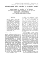
Collinearity analysis of the SNP loci between the genetic map and the physical map is shown in Fig 2. The
results indicated that the genetic map constructed by
the SNP markers which were discovered through SLAFseq had a sufficient coverage over the cotton genome.
Most of the SNP loci on the linkage map were in same
order as those on the corresponding chromosomes of
the physical map of the cotton genome. D subgenome
showed a better compatibility with the physical map as
compared to the A subgenome. Chromosomes 1, 2, 3,
5, 7, and11 in the A subgenome and chromosomes
14, 15, 16 and 18 in the D subgenome showed some
deviation in collinearity analysis (Additional file 4:
Table S4, Fig. 3).
The result of the RH analysis showed that among the
26 chromosomes, 21 have RHs, 9 and 12 of which were
in the A subgenome and D subgenome respectively.
Chromosome 13 harbored the largest number of 106 RHs
whereas the chromosomes 7, 15 and 18 only harbored
one RH. Chromosomes 3, 5, 8, 11 and 16 did not harbor
any RH. Additional information is shown in Additional file
5: Table S5, Fig. 4, and Table 3.

QTL mapping for boll weight in the RILs

A total of 146 QTLs for boll weight trait were detected
on 25 chromosomes across 11 environments (chromosome 8 was the exception). Sixteen of them were regarded
as stable QTLs as they could be detected in at least three

environments. In the confidence intervals of these stable
QTLs, qBW-chr13-7 harbored 26 markers whereas qBWchr02-3 and qBW-chr25-6 only harbored two markers.
Among these stable QTLs, qBW-chr13-7, detected in
seven environments, was located within the marker interval of CRI-SNP8685-CRI-SNP8731, and could explain
6.13–14.70 % of the observed phenotypic variation (PV).
QTL qBW-chr13-4, detected in six environments, was
located within the marker interval of CRI-SNP8313CRI-SNP-8346, and explained 4.58–6.06 % of the observed PV. QTLs qBW-chr01-1 and qBW-chr25-5, both
of which were detected in five environments, were
located within the marker intervals of CRI-SNP147CRI-SNP168 and CRI-SNP10564-CRI-SNP10569, and
explained 4.81–7.83 % and 4.29–10.76 % of the observed
PV respectively. QTLs qBW-chr02-3, qBW-chr07-1, qBWchr07-6, qBW-chr09-6 and qBW-chr25-7, all of which
were detected in four environments, located within the
marker intervals of CRI-SNP506-CRI-SNP519, CRI-SNP5634-CRI-SNP5581, CRI-SNP5454-CRI-SNP-5438, CRISNP6432-CRI-SNP6455 and CRI-SNP10592-CRI-SNP
10615, and explained 5.62–6.41, 4.95–8.89, 5.35–10.89,
5.01–10.31 and 7.58–7.80 % of the observed PV respectively. QTLs qBW-chr03-1, qBW-chr05-10, qBW-chr07-4,
qBW-chr16-4, qBW-chr22-3, qBW-chr23-5 and qBWchr25-6, all of which were detected in three environments,
were located within the marker intervals of CRI-SNP1241-CRI-SNP-1231, CRI-SNP-2294-CRI-SNP-2279, CRISNP-5497-CRI-SNP5472, CRI-SNP12560-CRI-SNP12270,
CRI-SNP10330-CRI-SNP10341, CRI-SNP13838-CRI-SNP
13865 and CRI-SNP10569-CRI-SNP10571, and explained
4.56–9.00, 5.64–7.45, 6.92–8.45, 4.15–5.03, 6.64–8.80,


Zhang et al. BMC Plant Biology (2016) 16:79

Page 7 of 18

Table 3 The detail information of the high-density genetic map
Chromosome
number

Marker
number

Total
distance

Average
distance

Chr01

297

140.42

0.47

Chr02

180

136.88

Chr03

218

159.93

Chr04

574

Chr05

434

Chr06
Chr07
Chr08
Chr09

Largest gap

P_value

SDR region

Number
of RHs

2.50

0.28

9

32

Number

of SDMs

4.48

0

82

0.76

5.42

1

12

6.67 %

1.36

0.44

1

35

0.73

4.15

0

47

21.56 %

2.36

0.40

4

0

142.01

0.25

3.61

0

27

4.70 %

1.14

0.43

0

86

242.56

0.56

4.22

0

106

24.42 %

2.46

0.29

10

0

101

92.62

0.92

4.76

0

26

25.74 %

2.37

0.43

1

16

318

132.96

0.42

3.56

0

36

11.32 %

1.58

0.35

1

1

56

45.12

0.81

3.56

0

13

23.21 %

2.32

0.26

0

0

274

156.33

0.57

5.07

1

60

21.90 %

2.30

0.32

5

55

Chr10

133

113.33

0.85

6.69

3

17

12.78 %

1.86

0.32

1

32

Chr11

88

112.62

1.28

5.71

1

24

27.27 %

2.50

0.30

3

0

Chr12

273

178.26

0.65

5.07

1

85

31.14 %

2.85

0.28

8

37

Chr13

604

185.33

0.31

4.15

0

44

7.28 %

1.43

0.40

1

106

Chr14

408

173.03

0.42

4.46

0

238

58.33 %

4.98

0.18

18

67

Chr15

29

41.39

1.43

3.56

0

8

27.59 %

2.76

0.33

1

1

Chr16

399

178.54

0.45

3.61

0

152

38.10 %

3.38

0.28

13

0

Chr17

102

101.64

1

4.79

0

9

8.82 %

1.28

0.43

0

29

Chr18

172

136.45

0.79

5.07

1

43

25.00 %

2.67

0.27

3

1

Chr19

109

94.13

0.86

4.76

0

18

16.51 %

2.10

0.35

2

24

Chr20

60

48.44

0.81

4.15

0

9

15.00 %

2.27

0.28

0

11

Chr21

174

163.73

0.94

5.71

1

29

16.67 %

1.77

0.43

2

40

Chr22

75

65.91

0.88

4.46

0

4

5.33 %

1.22

0.50

0

14

Chr23

142

127.61

0.9

4.76

0

31

21.83 %

2.26

0.32

3

36

Chr24

60

76.99

1.28

4.76

0

6

10.00 %

1.39

0.47

0

12

Chr25

166

124.21

0.75

5.39

1

84

50.60 %

4.62

0.16

6

39

Chr26

75

88.93

1.19

7.02

1

15

20.00 %

2.13

0.35

1

19

Total

5521

3259.37

0.78

7.02

11

1225

--

--

93

693

4.26–5.26 and 4.82–11.85 % of the observed PV respectively (Additional file 6: Table S6, Fig. 5, Table 4, Table 5).
The candidate genes annotation

In total, 344 candidate genes were identified in the
confidence intervals of stable QTLs. Except for the confidence interval of qBW-chr02-3 which has no candidate
gene, the confidence intervals of all the remaining QTLs
have candidate genes. The confidence intervals of qBWchr07-4 and qBW-chr25-6 harbored only one candidate
gene whereas the confidence interval of qBW-chr23-5
harbored 65 genes (Additional file 7: Figure S1, Additional
file 8: Figure S2). In total, 340 of the 344 candidate genes
had annotation information, among which 201, 81 and
163 had annotation information in GO, KEGG and KOG
respectively. In GO analysis, 435 genes were identified in
the cellular component category, 221 genes in the molecular function category, and 549 genes in the biological

Percentage
of SDMs

X2_value

Number of
gap (>5 cM)

27.61 %

--

process category, as some of the genes had multiple functions and could be categorized into two or more function

baskets. In the cellular component category, 102 genes
were related to cell and 101 genes were related to cell part.
In the molecular function category, 108 genes were related
to catalytic activity. In the biological process category, 133
genes were related to metabolic process and 108 genes
were related to cellular process (Additional file 9: Table
S7, Fig. 6). In the KEGG analysis, 81 genes were identified
in 55 pathways. Six genes were found in the plant hormone signal transduction pathway, four genes were found
in both the ribosome and protein processing pathways in
endoplasmic reticulum In all the remaining pathways,
there were no more than three genes found (Additional
file 10: Table S8, Additional file 11: Table S9). In the
KOG analysis, 24 genes only had the general prediction
function and 12 genes had unknown function. Among
the other 127 genes, 25 of them were related to


Zhang et al. BMC Plant Biology (2016) 16:79

Page 8 of 18

b

ch

r24

0
30
60

90
120
0
30
60
90
120

chr

hr25

G_chr26

23

4

0
30
60
9
12 0
1 0
0 50

1
r1

P_

G_c

30
60
90
120
0
30
60

G_

hr

60

60

Physical map

P_chr20
1

P_c
hr2

23

30

60
90
120
0
30
60

hr

9
12 0
0
0

_c

30
60
0

30
G

0
30
6
0 0
30
P_
c

0

30
60
0

ch

hr

0
30
60
90
12
15 0
0

hr18
G_c

G_chr19

Genenic map

Physical map

30
60

90
120
0
30
60
90
0
30
0
30
60
90
120
150
P_
ch
r22

r17

ch

G_

30
60
90
0

P_chr19

r22

30
60
90
120 0
15
0
30
60
90
120
150
180
12

P_chr1

3

3
6 0
90 0
0
30
60
90
120
150

0
30
60
90
120
150
180

0

0

30
60
90
0
30
60
90
120
0
30
60
90
0
30
0
30
60
90

120
150
0
30
60

ch

0

6

G_

G_

r1

hr21

P_
ch
r1
0

30 0
6 0
9
0

P_

G_
c

G_c
hr5

ch

8

G_c

P_chr
8

hr9

r
ch

P_

hr1

G_chr6

5

P _c

G_chr20

P_chr7

r8
G_ch

hr1

17

P_chr6

P_c

10

P_c

15
0

r5

9
chr
G_

4

r
ch
P_

30 0
6 0
9 20
1
0
30
60
90
120
150
180
210
240
0
30
60
90
0
30
60
90
120
0
30

0
30
60
90
12
15 0
0 0
3
6 0
90 0
0

P_chr1

90 0
12
0

3
6 0
9 0
12 0
0
0
30
60
9
1200
150
180

210
240
0
30
60
90
0
30
60
90
120
0
30
0
30
60
90
0
12 0
15 0
30
60
90

c
G_

h
P_c

G_chr7

r3

4

Genenic map

6

1
hr

ch

G_chr

0
30
60
90

P_

r
ch
P_

0
30

60 0
9
0
12 50
1 0

c
G_

G_

0
30
0

3
hr

14

15

chr

hr2

120
150

G_c

P_c

30
60
90
0
12

0
30
60
90
120
0
30
60
90
120

hr2

P_chr1

G_chr1

0
30
60
90

120
150
0
30

a

r24

ch

P_

5
chr2

P_chr26

P_

G_
ch
r1
1

12

chr

G_

G_chr13

Fig. 3 Collinearity between the genetic map and the physical map. a Collinearity of the A sub-genome between the genetic map and the physical
map. b Collinearity of the D sub-genome between the genetic map and the physical map

posttranslational modification, protein turnover, and
chaperones, 17 of them had a relation to signal transduction mechanisms, 12 of them had a relation to
translation, ribosomal structure and biogenesis, 11 of
them had a relation to carbohydrate transport and metabolism and 11 of them had a relation to transcription.
No more than 10 genes were found in other functions
in KOG classification (Fig. 6, Additional file 12: Table
S10, Additional file 13: Table S11, Table 5).
Among all 344 candidate genes, 44 were identified at
the nearest positions of the markers, of which the
genetic position had the highest LOD values in the QTL
mapping analysis (Additional file 7: Figure S1, Additional
file 8: Figure S2). Among them, 43 candidate genes had
annotation information except the gene Gh_D06G0216.
In the KEGG analysis, eight cand genes had annotation
information, five of which were related to hypothetical
protein, with the other three related s-adenosylmethionine
synthetase, polygalacturonase precursor and indole-3acetic acid-amido synthetase GH3.3 respectively. In KOG
analysis, 18 candidate genes had annotation information.
Two had unknown function, three were correlated to
signal transduction mechanisms, two were correlated to
translation, ribosomal structure and biogenesis, two were
correlated to posttranslational modification, protein turnover, and chaperones, two were correlated to inorganic
ion transport and metabolism, two were correlated to
secondary metabolites biosynthesis, transport and catabolism and two were correlated to carbohydrate transport

and metabolism. There was an additional gene correlated
to lipid transport and metabolism, one correlated to the
cytoskeleton, one correlated to coenzyme transport and

metabolism, one correlated to energy production and
conversion, one correlated to RNA processing and modification and one correlated to cell cycle control, cell division, and chromosome partitioning. In the GO analysis,
26 of the 43 had annotation information, among which,
21 were correlated to biological process, 21 were correlated to molecular function and 15 were correlated to
cellular component.

Discussion
The characteristics of the method SLAF-seq

For the simplified genome sequencing, the key step was
to make the simplified genome representative of the
whole genome. This was completed through the election
of suitable restriction endonuclease(s). When restriction
endonuclease(s) were applied to the genome digestion
and selected properly, the fragments generated by nextstep sequencing would be a better representation of the
genome. In the previous studies, usually a few common
restriction endonucleases such as EcoRI, SbfI and PstI
were used to digest the genome of various species [29].
Typically, only one restriction endonuclease was applied
to the genome digestion [30–32]. The genome specificity
of the species was ignored [29–33]. This might lead to
uneven distribution of the selected fragments in the
whole genome and thus make the simplified genome less
representative. Eventually the number of markers developed and reliability of the genetic map might both be
negatively affected [29, 33]. The SLAF-seq strategy, an
effective NGS-based method for large-scale SNP discovery and genotyping, has been applied successfully in

various species [12–14]. Compared with other tools for


Zhang et al. BMC Plant Biology (2016) 16:79

Page 9 of 18

chr01

chr02

chr03

chr04

chr05

chr06

chr07 chr08

chr09

chr10

chr11

chr12

chr13

chr14

chr15

chr16

chr17

chr18

chr19

chr20

chr22

chr23

chr24

chr25

chr26

chr21

Fig. 4 The genetic position of the recombination hotspots in the whole 26 chromosomes

large-scale genotyping with NGS technology, such as

RAD-seq and GBS, SLAF-seq displayed some unique
superiorities. First, the pre-design scheme with different
restriction endonuclease combinations was applied to
simulate in silico the result script of endonuclease digestions based on the sequencing database of A, D and AD
genomes of Gossypium [19, 34, 35] (Fig. 7). The

information on genomic GC content, repeat conditions
and genetic characteristics were referred to make up the
digestion strategy. After two endonucleases combinations
were applied to the genome digestion, the fragments ranging from 500 to 550 (including adapter) base pairs we
harvested for sequencing create a better representation of
the genome of Gossypium hirsutum L. Second, a dual-


Zhang et al. BMC Plant Biology (2016) 16:79

Page 10 of 18

Chr 02

Chr 01
LOD

Exp(%)
8
7

3

Chr 03

Exp(%)
7

LOD
3

6

6
LOD=2.3

5

2

Exp(%)
10

LOD
5

8

4

5
LOD=2.1

2

4

6

3

4
3
3

1

2

1

0
0

20

40

60
80
100 120
genetic distance (cM)

1
0

140

2

4

1

2

2

1
0

LOD=2.2

0

20

40

60

80

100

0
140

120

0
0

20

40

genetic distance (cM)

Chr 05
Exp(%)
8

80

100 120

0
160

140

genetic distance (cM)

Chr 07

LOD
4

60

Chr 09

LOD

Exp(%)

4

8

Exp(%)
12

LOD
5

10

7
3

6
LOD=2.3

4

3

2

4

3

LOD=2.0

2

2

6

4

3
1

8

6

5

1

2

LOD=2.2
2

4

1

2

1
0

0

50

100
150
200
genetic distance (cM)

0
250

0
0

20

40
80
100
60
genetic distance (cM)

120

0
140

0
0

20

Chr 16

Chr 13
Exp(%)

LOD
4

8

6
LOD=2.3

2

0
160

140

LOD

Exp(%)

3
6

5
LOD=2.1

2

4

5

2

4

4

3
1

1

80 100 120
60
genetic distance (cM)

Chr 22
Exp(%)
7

LOD

LOD=2.3
3

40

3
1

2

2

2

1

1
0

0
0

50

Chr 23

LOD

0

100
150
genetic distance (cM)
Exp(%)
6

0

20

40

0
60 80 100 120 140 160 180
genetic distance (cM)

Chr 25

LOD

0

0
0

10

20
30
40
50
genetic distance (cM)

60

Exp(%)
14

6
12

5
5

LOD=2.0

2

10

4
4
3

1

2
1

0

0

20

40

60
80
100
genetic distance (cM)

120

0

140

8

3

6
LOD=2.1

2

4

1

2

0

0
0

20

40
60
80
100
genetic distance (cM)

LOD
Exp(%)

120

Fig. 5 The LOD value and the observed PV value of the stable QTLs

index will provide a higher sequence quality and more
stable sequence depth among each sample, which is the
key to developing high quality marker. Third, the marker
underwent a series of dynamic processes to discard the

suspicious markers during each cycle, until the average
genotype quality score of all SLAF markers reached the
cut-off value. As a result, the markers we developed might
have a consistent distribution throughout the genome and


QTL name

Environment Position LOD Additive R2

Marker interval (P < 0.01)

Marker interval (P < 0.05)

qBW-chr01-1

10GY

45.41

2.43

0.25

5.32 %

CRI-SNP161-CRI-SNP168

CRI-SNP147-CRI-SNP168

07AY

46.41

2.20

0.20

08AY

47.41

2.52

0.18

08LQ

47.41

3.35

08QZ

47.41

3.44

qBW-chr02-3

qBW-chr03-1

qBW-chr07-6

qBW-chr09-6

47.00

44.30

47.70

4.81 %

46.00

47.70

45.40

50.30

5.19 %

45.10

48.20

42.50

50.30

0.19

7.05 %

46.00

49.50

44.70

50.30

0.28

7.83 %

45.60

49.20

45.40

50.30

08AY

21.11

2.82

0.15

6.15 %

21.11

2.52

0.15

5.62 %

CRI-SNP511-CRI-SNP512

CRI-SNP506-CRI-SNP519

20.70

23.00

20.70

25.10

19.70

23.00

18.40

25.10

08QZ

21.11

2.85

0.16

6.41 %

20.70

22.50

19.40

24.30

10AY

21.11

2.57

0.15

5.67 %

19.30

23.80

18.40

27.30

08AY

34.01

4.50

0.16

9.00 %

08LQ

34.01

3.85

0.16

8.29 %

10AY

qBW-chr07-4

45.10

08LQ

34.01

2.28

0.11

4.56 %

195.81

3.52

−0.16

7.45 %

07AY

199.21

3.50

−0.11

13AY

199.21

2.85

−0.16

09AKS

31.51

3.97

0.17

8.89 %

08AY

32.01

2.85

0.20

6.32 %

qBW-chr05-10 09AKS

qBW-chr07-1

LOD_L (P < 0.01) LOD_R (P < 0.01) LOD_L (P < 0.05) LOD_R (P < 0.05)

CRI-SNP-1241-CRI-SNP-1235

CRI-SNP-1241-CRI-SNP-1231

32.60

34.80

31.40

34.80

33.40

35.80

33.20

38.10

31.40

36.80

31.40

45.30

195.00

197.50

195.00

197.90

7.43 %

199.00

200.50

197.60

200.50

5.64 %

199.10

200.30

197.60

200.50

CRI-SNP-2294-CRI-SNP-2279

CRI-SNP-5633-CRI-SNP5596

CRI-SNP-2294-CRI-SNP-2279

CRI-SNP-5634-CRI-SNP5581

30.40

32.10

30.40

32.20

31.40

32.80

30.00

33.50

08QZ

32.01

2.41

0.20

4.95 %

31.40

32.50

31.40

32.50

09AY

32.01

3.80

0.19

8.07 %

31.40

32.30

29.60

33.00

13AY

50.61

3.66

−0.24

7.64 %

09QZ

51.11

3.34

−0.23

6.92 %

CRI-SNP5490-CRI-SNP5481

CRI-SNP-5497-CRI-SNP5472

50.10

51.10

49.80

51.10

50.10

52.30

49.30

53.20

50.30

51.50

50.10

51.60

57.80

59.30

56.80

60.10

10AY

51.11

4.08

−0.23

8.45 %

10AY

58.61

4.38

−0.22

9.03 %

10ZZ

58.61

5.21

−0.28

10.89 %

57.80

59.20

57.80

59.70

09QZ

59.11

2.55

−0.19

5.35 %

57.80

60.20

57.80

60.70

CRI-SNP5452-CRI-SNP-5441

13AY

60.21

2.58

−0.19

5.45 %

07AY

114.11

4.77

−0.14

10.31 % CRI-SNP6432-CRI-SNP6455

CRI-SNP5454-CRI-SNP-5438

CRI-SNP6432-CRI-SNP6455

59.90

60.50

59.90

60.80

113.70

115.40

112.80

115.40

114.11

2.44

−0.13

5.01 %

113.00

116.70

112.80

116.70

09AKS

114.11

2.75

−0.16

5.80 %

112.70

114.60

112.00

114.60

09AY

114.61

3.27

−0.14

6.54 %

112.90

115.40

112.80

115.40

Page 11 of 18

09QZ

Zhang et al. BMC Plant Biology (2016) 16:79

Table 4 The detail information about the stable QTLs


qBW-chr13-4

qBW-chr13-7

qBW-chr16-4

qBW-chr22-3

qBW-chr23-5

qBW-chr25-5

qBW-chr25-6

08LQ

58.71

2.43

−0.12

4.58 %

13AY

60.01

2.55

−0.17

09AY

62.81

2.33

−0.11

07AY

64.51

2.99

08AY

64.51

2.76

CRI-SNP8317-CRI-SNP-8338

CRI-SNP8313-CRI-SNP-8346

57.40

60.00

56.10

60.00

5.24 %

58.60

63.10

58.20

66.30

5.05 %

58.10

66.30

57.90

70.10

−0.12

6.06 %

63.70

66.80

63.70

68.30

−0.13

5.17 %

63.70

67.80

63.70

68.90

10AY

64.51

2.46

−0.12

4.87 %

09AKS

114.61

2.95

0.34

6.13 %

08LQ

114.91

8.37

0.52

08QZ

115.11

7.21

0.50

10AY

115.11

4.14

0.38

8.36 %

114.90

115.40

114.60

115.50

08AY

115.41

6.97

0.49

13.72 %

114.90

115.90

114.90

115.70

62.10

66.80

58.70

68.90

113.90

115.90

113.20

116.50

16.70 %

114.60

115.30

114.50

115.50

14.76 %

114.70

116.20

114.50

115.80

CRI-SNP8690-CRI-SNP8726

CRI-SNP8685-CRI-SNP8731

09QZ

115.41

2.99

0.34

6.45 %

114.60

116.30

114.30

117.30

07AY

115.61

4.03

0.33

8.21 %

115.40

117.10

115.40

116.50

09AY

80.21

2.97

−0.14

6.46 %

10AY

80.21

4.12

−0.22

8.48 %

CRI-SNP12560-CRI-SNP12271 CRI-SNP12560-CRI-SNP12270

79.40

81.00

79.40

81.20

79.80

84.30

79.40

83.30

82.00

86.00

82.00

87.00

51.00

54.20

49.20

56.80

07AY

83.01

3.25

−0.13

6.85 %

09AY

52.61

2.10

−0.10

4.52 %

10GY

55.81

1.97

−0.10

4.15 %

51.00

59.90

55.80

55.80

10AY

55.81

2.25

−0.11

5.03 %

54.20

58.30

54.20

58.90

08AY

101.81

2.14

0.12

4.26 %

10ZZ

102.61

2.46

0.16

5.26 %

08QZ

103.61

2.40

0.13

5.17 %

08AY

22.41

4.39

0.19

9.36 %

10ZZ

22.41

5.17

0.25

08LQ

22.51

2.20

0.13

09AY

23.51

4.08

09QZ

25.41

2.52

CRI-SNP10333-CRI-SNP10341 CRI-SNP10330-CRI-SNP10341

CRI-SNP13840-CRI-SNP13862 CRI-SNP13838-CRI-SNP13865

98.00

106.50

96.80

107.30

99.00

105.00

96.90

105.80

100.90

104.70

97.00

105.80

20.40

23.50

20.40

24.40

10.76 %

20.40

24.20

20.40

26.30

4.29 %

20.40

26.40

20.40

27.10

0.18

9.26 %

20.40

24.40

20.30

24.40

0.17

6.11 %

23.80

29.20

23.50

29.20

CRI-SNP10565-CRI-SNP10569 CRI-SNP10564-CRI-SNP10569

10ZZ

28.11

3.06

0.20

7.08 %

27.10

32.80

27.10

32.80

09AY

30.81

5.68

0.21

11.85 %

CRI-SNP10569-CRI-SNP10568 CRI-SNP10569-CRI-SNP10571

27.70

32.50

24.40

32.90

09QZ

30.81

2.17

0.15

4.82 %

29.20

32.50

29.20

32.90

Zhang et al. BMC Plant Biology (2016) 16:79

Table 4 The detail information about the stable QTLs (Continued)

Page 12 of 18


qBW-chr25-7

10GY

45.91

3.51

−0.22

7.79 %

10AY

45.91

3.83

−0.15

09AY

49.61

3.83

−0.15

10ZZ

52.71

3.63

−0.18

CRI-SNP10592-CRI-SNP10614 CRI-SNP10592-CRI-SNP10615

44.90

47.60

44.40

47.00

7.70 %

44.70

48.00

44.40

48.00

7.80 %

48.30

53.00

48.00

53.50

7.58 %

52.50

53.20

52.50

53.20

Zhang et al. BMC Plant Biology (2016) 16:79

Table 4 The detail information about the stable QTLs (Continued)

Page 13 of 18


Zhang et al. BMC Plant Biology (2016) 16:79

Page 14 of 18

Table 5 The markers and the candidate genes in the confidence intervals of the stable QTLs
QTL name

Marker interval (P < 0.01)

Gene interval

Physical distance interval

Number of markers

Number of genes

qBW-chr01-1

CRI-SNP161-CRI-SNP168

CRI-SNP161-CRI-SNP166

21363529–22191102

5

8

qBW-chr02-3

CRI-SNP511-CRI-SNP512

CRI-SNP511-CRI-SNP512

2428231–2465227

2

None

qBW-chr03-1

CRI-SNP-1241-CRI-SNP-1235

CRI-SNP-1241-CRI-SNP-1235

93109282–93363954

6

3

qBW-chr05-10

CRI-SNP-2294-CRI-SNP-2279

CRI-SNP-2294-CRI-SNP-2281

11840100–12807341

11

51

qBW-chr07-1

CRI-SNP-5633-CRI-SNP5596

CRI-SNP-5633-CRI-SNP5596

41686619–43069600

18

15

qBW-chr07-4

CRI-SNP5490-CRI-SNP5481

CRI-SNP5490-CRI-SNP5481

26629060–26694814

10

1

qBW-chr07-6

CRI-SNP5452-CRI-SNP-5441

CRI-SNP5452-CRI-SNP-5441

26153119–26450470

7

11

qBW-chr09-6

CRI-SNP6432-CRI-SNP6455

CRI-SNP6432-CRI-SNP6455

55762226–57316457

15

28

qBW-chr13-4

CRI-SNP8317-CRI-SNP-8338

CRI-SNP8317-CRI-SNP-8338

5157441–5989840

13

34

qBW-chr13-7

CRI-SNP8690-CRI-SNP8726

CRI-SNP8690-CRI-SNP8726

41941944–43033838

26

10

qBW-chr16-4

CRI-SNP12271-CRI-SNP12560

CRI-SNP12483-CRI-SNP12560

15223879–15984482

19

37

qBW-chr22-3

CRI-SNP10333-CRI-SNP10341

CRI-SNP10333-CRI-SNP10341

47103662–47711028

8

39

qBW-chr23-5

CRI-SNP13840-CRI-SNP13862

CRI-SNP13840-CRI-SNP13862

43266988–43944781

7

65

qBW-chr25-5

CRI-SNP10565-CRI-SNP10569

CRI-SNP10565-CRI-SNP10569

1826714–2154361

5

32

qBW-chr25-6

CRI-SNP10569-CRI-SNP10568

CRI-SNP10569-CRI-SNP10568

2129899–2154631

2

1

qBW-chr25-7

CRI-SNP10592-CRI-SNP10614

CRI-SNP10592-CRI-SNP10614

2861896–3087983

10

10

the thus-built map might have a better coverage of the
genome and be more reliable for the next step research
activities.
Genetic map construction

In previous studies, most of the genetic maps of cotton
were based SSR markers. The low polymorphic rate of
the SSR markers makes the SSR marker based maps
unable to harbor a sufficient number of markers with a
comparative poor coverage of the genome and low

resolution. In most cases, these maps have large gaps,
and sometimes the gap divides the chromosome into
two or more linkage groups [16, 36, 37]. When the populations developed from interspecific crosses between
G. hirsutum and G. barbadense were applied to the
genetic map construction, the coverage and resolution
of the map could be greatly improved [38–40]. However, the pragmatic applications of the genetic map
developed from the interspecific populations have limited values as the polymorphic loci between G. hirsutum and G. barbadense may not show polymorphism
within the cultivars of G. hirsutum. SNP markers could
improve the coverage and resolution of the genetic map
efficiently. Wang et al. [4] used SNP markers to construct a map through the RAD-seq, which harbored
3984 markers with a total distance of 3499.69 cM and
an average distance of 0.88 cM. In our research, we
constructed an HDGM through the SNP markers developed through the SLAF-seq method. Even though
the map harbored a great number of markers and was
more saturated than most of the previous ones, the
total distance it covered was approximately the same as

the previous studies. Some of the chromosomes only
spanned very short genetic distances on the map. The
shortest three chromosomes (chromosomes 15, 8 and
20) only spanned 41.39 cM, 45.12 cM and 48.44 cM,
harboring 29, 56 and 60 markers respectively. Previous
studies showed that different populations might generate varied chromosome genetic distances of the Gossypium hirsutum genome. In the initial steps of marker
development through SLAF-seq, the quantities of SLAFs
developed were about the same sizes in the different chromosomes. After several steps of screenings, the remaining
numbers of SNPs for map construction varied greatly
among the chromosomes, and the reduced number of
remaining SNPs contributed to the shortness of some
chromosomes. The collinearity comparison between the
genetic map and the physical one validates the reliability

of the constructed map. However, a better understanding
of the genetic structure of these chromosomes might need
an integrative analysis.
The QTL of boll weight traits identification

Previous QTL studies were primarily focused on the
fiber quality traits [1, 2, 40], while the research activities
on yield traits especially the boll weight were seldom
reported. The boll weight trait was significant and made
a considerable contribution to the yield of cotton. Qin et
al. [41] used the four-way cross (4WC) population to
construct a map and identified only one QTL of boll
weight on chromosome D2. The confidence interval of
this QTL harbored three markers and spanned a distance
of about 14.5 cM. Liu et al. [42] used RIL population to
construct a map and identified the QTL of boll weight


Zhang et al. BMC Plant Biology (2016) 16:79

Page 15 of 18

a
211

biologic
al phase

cess

process
rganism

multi-o

uction

stem p
ro

immun
e sy

growth

reprod

transpo

nucleic

acid bin

ding tra

macrom
olecula

membra
n

organe

organe

cell

binding
rter act
ivity
nscriptio
n facto
r activity
structu
ral mole
cule act
ivity
electro
n carrie
r activity
antioxi
dant act
ivity
molecu
lar tran
sducer
activity
enzym
e regula
tor activ

ity
metabo
lic proce
ss
cellular
process
single-o
rganism
process
biologic
al regu
lation
respon
se to st
imulus
localiza
tion
develo
cellular
pmenta
compo
l proce
nent org
ss
anizatio
n or bio
genesi
s
signalin
multice

g
llular o
rganism
al proce
ss
reprod
uctive
process

0

r comp
lex
membra
ne part
extrace
llular re
gion
cell jun
ction
catalytic
activity

0.1

e

2

lle part

1

rt

21

lle

10

Number of genes

Cotton.longest trans

cell pa

Percent of genes

100

Cellular component

Molecular function

Biological process

b
A: RNA processing and modification
B: Chromatin structure and dynamics

C: Energy production and conversion
D: Cell cycle control, cell division, chromosome partitioning
E: Amino acid transport and metabolism
F: Nucleotide transport and metabolism
G: Carbohydrate transport and metabolism
H: Coenzyme transport and metabolism
I: Lipid transport and metabolism
J: Translation, ribosomal structure and biogenesis
K: Transcription
L: Replication, recombination and repair
M: Cell wall/membrane/envelope biogenesis
O: Posttranslational modification, protein turnover, chaperones
P: Inorganic ion transport and metabolism
Q: Secondary metabolites biosynthesis, transport and catabolism
R: General function prediction only
S: Function unknown
T: Signal transduction mechanisms
U: Intracellular trafficking, secretion, and vesicular transport
V: Defense mechanisms
W: Extracellular structures
Z: Cytoskeleton

Frequency

20

10

0
A

B

C

D

E

F

G

H

I

J

K

L

M

O

P

Q

R

S

T

U

V

W

Z

Function Class

Fig. 6 The annotation of the candidate genes in the confidence intervals of the stable QTLs. a The annotation of the candidate genes in the
confidence intervals of the QTLs that could be detected in at least three environments through GO analysis. b The annotation of the candidate
genes in the confidence intervals of the QTLs that could be detected in at least three environments through KOG analysis

using the mean value of the data from four environments.
Eighteen QTLs for boll weight were detected on 15
chromosomes. The confidence intervals of these QTLs
harbored two or three markers. Yu et al. [43] used an
interspecific backcross inbred line (BIL) population

developed with a G. hirsutum and a G. barbadense to construct a genetic map and identified 10 QTLs on eight
chromosomes (chromosomes 5, 11, 18, 21, 22, 24, 25, and
26). The confidence intervals of these QTLs also harbored

two or three markers and spanned distances from 2 to


Zhang et al. BMC Plant Biology (2016) 16:79

b

Genome-wide distribution of read coverage
10
0
10
0
10
0
10
0
10
0
10
0
10
0
10
0
10
0
10
0
10
0

10
0
10
0
10
0
10
0
10
0
10
0
10
0
10
0
10
0
10
0
10
0
10
0
10
0
10
0
10
0

0kb

Chr01
Chr02
Chr03
Chr04
Chr05
Chr06
Chr07
Chr08
Chr09
Chr10
Chr11
Chr12
Chr13
Chr14
Chr15
Chr16
Chr17
Chr18
Chr19
Chr20
Chr21
Chr22
Chr23
Chr24
Chr25
Chr26

2500kb

5000kb

7500kb

10000kb

Chromsome position

Median of read deinsity(log(2))

Median of read deinsity(log(2))

a

Page 16 of 18

Genome-wide distribution of read coverage
10
0
10
0
10
0
10
0
10
0
10

0
10
0
10
0
10
0
10
0
10
0
10
0
10
0
10
0
10
0
10
0
10
0
10
0
10
0
10
0
10

0
10
0
10
0
10
0
10
0
10
0

Chr01
Chr02
Chr03
Chr04
Chr05
Chr06
Chr07
Chr08
Chr09
Chr10
Chr11
Chr12
Chr13
Chr14
Chr15
Chr16
Chr17
Chr18

Chr19
Chr20
Chr21
Chr22
Chr23
Chr24
Chr25
Chr26

0kb

500kb

1000kb

1500kb

2000kb

Chromsome position

Fig. 7 Genome-wide distribution of reads coverage. a Genome-wide distribution of reads coverage with window size of 10 K. b Genome-wide
distribution of reads coverage with window size of 50 K

30 cM. In our study, we identified the QTL of the boll
weight in 25 chromosomes except chromosome 8. Among
them 16 QTLs were detected in at least three environments and were present on 11 chromosomes (chromosomes 1, 2, 3, 5, 7, 9, 13, 16, 22, 23, and 25 respectively).
The confidence intervals of these QTLs harbored from
two to 26 markers ranging from 0.7 to 13.9 cM. This implies that our results of QTL identification are more concise and accurate than previous studies and could be
useful for future research looking at gene identification or

cloning from these QTLs, or even breeding practices
using MAS.
The direction of the QTLs

Among the 16 stable QTLs that can be detected in at least
three environments, eight had positive additive effects
whereas the other eight had negative additive effects. This
indicates that both the higher boll weight value parent
sGK9708 and lower boll weight value parent 0–153 could
contribute positive additive QTLs to increase the boll
weight. This could be a possible factor behind the difference in the boll weight trait between the parents 0–153
and sGK9708. Theoretically, the greater the difference of
one trait between the two parents, the higher the possibility that the positive additive effect of the QTLs would
come from one parent. The RIL population was constructed primarily based on differences in fiber quality
traits especially fiber strength between the parents 0–153
and sGK9708, therefore, the difference of fiber strength
is larger than that of any other traits between 0–153
and sGK9708. In Sun’s report [16], seven QTLs of fiber
strength were identified using this population, among
which only one QTL had negative additive effects whereas

the remaining six QTLs had positive additive effects. In
Zhang’s report [17], seven QTLs of fiber strength on
chromosome 25 were identified using the same population, all of which had a positive additive effect. In identifying the QTL clusters, the clusters that harbor all
desired QTL alleles would make the greater contribution to the breeding practice when MAS is applied.
Candidate gene functioning analysis

Among all 340 candidate genes being annotated in at
least one channel of KOG, KEGG, and GO, some might
be related to the boll weight trait. In KOG analysis, there

were 21 function baskets. The posttranslational modification function, protein turnover, chaperones and signal
transduction mechanisms harbored the largest number
of candidate genes. Among the 44 genes located closest to the markers of genetic position, three genes
Gh_A07G1188, Gh_A07G1197and Gh_D09G1606 had
a relation to signal transduction mechanisms. Two
genes, Gh_A05G1210 and Gh_D04G1531 were related
the function posttranslational modification, protein turnover, and chaperones. Two genes, Gh_A07G1187 and
Gh_A13G0858, had the translation function, ribosomal
structure, and biogenesis, though this function basket did
not harbor a large number of candidate genes. As the
posttranslational modification, protein turnover and ribosomal structure were relative to the protein synthesis, it is
probable that the genes correlated to this function contribute to the boll weight trait.
In KEEG analysis, the first three pathways which harbored the largest number of genes were plant hormone
signal transduction, and protein processing in endoplasmic reticulum and ribosome, harboring six genes, four


Zhang et al. BMC Plant Biology (2016) 16:79

genes and four genes respectively. Of these 14 genes, three
were located at the nearest positions of the markers, genetic position of which had the highest LOD values in
the QTL mapping analysis. The gene Gh_A13G0858
has a relationship to the ribosome, whereas genes
Gh_A13G0392 and Gh_D06G0187 have a relationship
to the plant hormone signal transduction. As the ribosome has a relationship to protein synthesis and some
plant hormones such as auxin and gibberellin, these
genes could contribute to the plant growth and eventually to the boll weight trait, particularly the gene
Gh_A13G0858.
Although these genes were located the nearest position
of the markers, genetic position of which had the highest
LOD values in the QTL mapping analysis, but there still

lacks direct evidence to prove that the function of these
genes was correlated to the boll weight trait.

Conclusions
This research reported the first HDGM of Upland Cotton
(Gossypium hirsutum) with a RIL population using SNP
markers developed by SLAF-seq. The HDGM had a
total number of 5521 markers and a total distance of
3259.37 cM with an average marker interval of 0.78 cM.
There were no gaps greater than 10 cM.We also identified
QTLs of boll weight trait across 11 environments and
identified candidate genes. Totally, 146 QTLs of boll
weight was identified and 16 of them were detected in at
least three environments with a stable QTL. Three hundred forty-four candidate genes were identified in the
confidence intervals of stable QTLs and 44 of them were
located in the nearest positions of the markers. The result
of this research would provide information for the next
phase of research such as fine mapping, gene functional
analysis, pyramiding breeding and marker-assisted selection (MAS) as well.
Availability of supporting data

The data sets supporting the results of this article are
included within the article and its additional files.

Additional files
Additional file 1: Table S1. Distribution of the SNP markers’ type on
the genetic map. (XLSX 9 kb)
Additional file 2: Table S2. The markers and their genetic distance in
the genetic map. (XLSX 149 kb)
Additional file 3: Table S3. The X2_value and P_value of all the

markers in the genetic map. (XLSX 233 kb)
Additional file 4: Table S4. The physical position of all the markers in
the genetic map. (XLSX 213 kb)
Additional file 5: Table S5. The genetic position of all the recombination
hotspots in the genetic map. (XLSX 34 kb)
Additional file 6: Table S6. All the QTLs identified including the ones
that can be detected only in one environment. (XLSX 29 kb)

Page 17 of 18

Additional file 7: Figure S1. The physical map of the SNP markers and
the candidate genes in the confidence intervals of the stable QTLs in A
sub-genome. Footnote: Red: The candidate genes. Blue: The SNP markers.
★: The SNP markers that located in the nearest genetic position of the
highest LOD value in QTL analysis. ●: The candidate genes that located in
the nearest genetic position of the highest LOD value in QTL analysis.
(PNG 959 kb)
Additional file 8: Figure S2. The physical map of the markers and
the candidate genes in the confidence intervals of the stable QTLs in D
sub-genome. Footnote: Red: The candidate genes. Blue: The SNP markers.
★: The SNP markers that located in the nearest genetic position of the
highest LOD value in QTL analysis. ●: The candidate genes that located in
the nearest genetic position of the highest LOD value in QTL analysis.
(PNG 827 kb)
Additional file 9: Table S7. The GO annotation result of the candidate
genes of the stable QTLs of cotton boll weight. (XLSX 13 kb)
Additional file 10: Table S8. The KEGG annotation result of all the
candidate genes of the stable QTLs of cotton boll weight. (XLSX 15 kb)
Additional file 11: Table S9. The number of the candidate genes and
the genes ID in each pathway in the KEGG annotation (XLSX 13 kb)

Additional file 12: Table S10. The KOG annotation result all the
candidate genes of the stable QTLs of cotton boll weight. (XLSX 15 kb)
Additional file 13: Table S11. The number of the candidate genes in
each function categories of the KOG annotation. (XLSX 11 kb)

Competing interests
The authors declare that they have no competing interests.
Authors’ contribution
ZZ, JWL, QG, JWG, AYL and TTC do the experiment of the library
construction and sequencing. HHS, DW, PKK, MJ, WJL, QWL and YLW collect
the data from the field. YZS, LH, XYD, YNT, WWS, CJ, PTL and RHO analyze
the data. WKG, ZZ and LH prepare the manuscript. WKG and YLY design the
experiment and provide the materials. All authors have read, edited and
approved the current version of the manuscript.
Acknowledgments
This work was funded by the Natural Science Foundation of China
(31371668, 31471538), the National High Technology Research and
Development Program of China (2012AA101108), the National Agricultural
Science and technology innovation project for CAAS and the Henan
province foundation with cutting-edge technology research projects
(142300413202). The funders had no role in study design, data collection
and analysis, decision to publish, or preparation of the manuscript.
Author details
1
State Key Laboratory of Cotton Biology, Key Laboratory of Biological and
Genetic Breeding of Cotton, The Ministry of Agriculture, Institute of Cotton
Research, Chinese Academy of Agricultural Sciences, Anyang 455000, Henan,
China. 2Biomarker Technologies Corporation, Beijing 103100, China. 3Anyang
Institute of Technology, Anyang 455000, Henan, China.
Received: 9 December 2015 Accepted: 17 February 2016

References
1. Shen XL, Guo WZ, Zhu XF, Yuan YL, Yu JZ, Kohel JR, et al. Molecular
mapping of QTLs for fiber qualities in three diverse lines in Upland cotton
using SSR markers. Mol Breeding. 2005;15:169–81.
2. Zhang K, Zhang J, Ma J, Tang SY, Liu DJ, Teng ZH, et al. Genetic mapping
and quantitative trait locus analysis of fiber quality traits using a threeparent composite population in upland cotton (Gossypium hirsutum L.). Mol
Breeding. 2012;29:335–48.
3. Ning ZY, Chen H, Mei HX, Zhang TZ. Molecular tagging of QTLs for fiber
quality and yield in the upland cotton cultivar Acala-Prema. Euphytica.
2014;195:143–56.


Zhang et al. BMC Plant Biology (2016) 16:79

4.

5.

6.

7.

8.

9.

10.

11.

12.

13.

14.

15.

16.

17.

18.

19.

20.
21.

22.
23.
24.

Wang YK, Ning ZY, Hu Y, Chen JD, Zhao R, Chen H, et al. Molecular
Mapping of Restriction-Site Associated DNA Markers in Allotetraploid
Upland Cotton. PLoS One. 2015;10(4), e0124781.
Wei QZ, Wang YZ, Qin XD, Zhang YX, Zhang ZT, Wang J, et al. An SNPbased saturated genetic map and QTL analysis of fruit-related traits in
cucumber using specific–length amplified fragment (SLAF) sequencing.
BMC Genomics. 2014;15:1158.

Cai CF, Cheng FY, Wu J, Zhong Y, Liu CX. The First High-Density
Genetic Map Construction in Tree Peony (Paeonia Sect.Moutan) using
Genotyping by Specific-Locus Amplified Fragment Sequencing. PLoS
One. 2014;10(5):e0128584.
Guo SY, Shi GL, Liu ZD, Zhao YH, Yang XX, Zhu JC, et al. Using specific
length amplified fragment sequencing to construct the high-density
genetic map for Vitis (Vitis vinifera L. × Vitis amurensis Rupr.). Front Plant Sci.
2015; doi:10.3389
Baird NA, Etter PD, Atwood TS, Currey MC, Shiver AL, Lewis ZA, et al. Rapid
286 SNP discovery and genetic mapping using sequenced RAD markers.
PLoS One. 2008;3(10), e3376.
Elshire RJ, Glaubitz JC, Sun Q, Poland JA, Kawamoto K, Buckler ES, et al.
A 297 robust, simple genotyping-by-sequencing (GBS) approach for high
diversity species. PLoS One. 2011;6(5), e19379.
Sun XW, Liu DY, Zhang XF, Li WB, Liu H, Hong WG, et al. SLAF–seq: An
Efficient Method of Large–Scale De Novo SNP Discovery and Genotyping
Using High–Throughput Sequencing. PLoS One. 2013;8(3), e58700.
Zhang YX, Wang LH, Xin HG, Li DH, Ma CX, Ding X, et al. Construction
of a high-density genetic map for sesame based on large scale marker
development by specific length amplified fragment (SLAF) sequencing.
BMC Plant Biol. 2013;13:141.
Ma JQ, Huang L, Ma CL, Jin JQ, Li FC, Wang KR, et al. Large–Scale SNP
Discovery and Genotyping for Constructing a High-Density Genetic Map of
Tea Plant Using Specific–Locus Amplified Fragment Sequencing (SLAF-seq).
PLoS ONE. 2015;10(6), e0128798.
Zhang J, Zhang QX, Cheng TR, Yang WR, Pan HT, Zhong JJ, et al. High–
density genetic map construction and identification of a locus controlling
weeping trait in an ornamental woody plant (Prunus mume Sieb. et Zucc).
DNA Research. 2015;22(3):183–91.
Xu XW, Xu RX, Zhu BY, Yu T, Qu WQ, Lu L, et al. A High–Density Genetic

Map of Cucumber Derived from Specific Length Amplified Fragment
sequencing (SLAF-seq). Front Plant Sci. 2014; doi: 10.3389
Li B, Tian L, Zhang JY, Huang L, Han FX, Yan SR, et al. Construction of a
high–density genetic map based on large–scale markers developed by
specific length amplified fragment sequencing (SLAF-seq) and its
application to QTL analysis for isoflavone content in Glycine max. BMC
Genomics. 2014;15:1086.
Sun FD, Zhang JH, Wang SF, Gong WK, Shi YZ, Liu AY, et al. QTL mapping
for fiber quality traits across multiple generations and environments in
upland cotton. Mol Breeding. 2012;30:569–82.
Zhang Z, Li JW, Muhammad J, Cai J, Jia F, Shi YZ, et al. High Resolution
Consensus Mapping of Quantitative Trait Loci for Fiber Strength, Length
and Micronaire on Chromosome 25 of the Upland Cotton (Gossypium
hirsutum L.). PLoS One. 2015;10(8), e0135430.
Li FG, Fan GY, Lu CR, Xiao GH, Zou CS, Kohel RJ, et al. Genome sequence
of cultivated Upland cotton (Gossypium hirsutum TM–1). Nat Biotechnol.
2015;33:524–30.
Zhang TZ, Hu Y, Jiang WK, Fang L, Guan XY, Chen JD, et al. Sequencing of
allotetraploid cotton (Gossypium hirsutum L. acc. TM–1) provides a resource
for fiber improvement. Nature Biotechnol. 2015;33:531–7.
Li H, Durbin R. Fast and accurate short read alignment with BurrowsWheeler Transform. Bioinformatics. 2009;25:1754–60.
Liu DY, Ma CX, Hong WG, Huang L, Liu M, Zeng HP, et al. Construction and
Analysis of High-Density Linkage Map Using High-Throughput Sequencing
Data. PLoS ONE. 2014;9(6), e98855.
Jansen J, de Jong AG, van Ooijen JW. Constructing dense genetic linkage
maps. Theor Appl Genet. 2001;102:1113–22.
van Ooijen JW. Multipoint maximum likelihood mapping in a full-sib family
of an outbreeding species. Genetics research. 2011;93:343–9.
van Os H, Stam P, Visser RG, van Eck HJ. SMOOTH: a statistical method for
successful removal of genotyping errors from high-density genetic linkage

data. Theoretical and Applied Genetics. 2005;112:187–94.

Page 18 of 18

25. Huang XH, Zhao Y, Wei XH, Li CY, Wang AH, Zhao Q, et al. Genome-wide
association study of flowering time and grain yield traits in a worldwide
collection of rice germplasm. Nature Genetics. 2012;44(1):32–9.
26. Kosambi DD. The estimation of map distance from recombination values.
Ann Eugen. 1944;12:172–5.
27. Wang S, Basten CJ, Zeng ZB. Windows QTL Cartographer 2.5. Department of
Statistics, North Carolina State University, Raleigh, NC. 2001. http://statgen.
ncsu.edu/qtlcart/WQTLCart.htm. Accessed 2013 Feb 1.
28. Zeng ZB. Precision mapping of quantitative trait loci. Genetics. 1994;136:1457–68.
29. Barchi L, Lanteri S, Portis E, Valè GA, Volante A, Pulcini L, et al. A RAD Tag
Derived Marker Based Eggplant Linkage Map and the Location of QTLs
Determining Anthocyanin Pigmentation. PLoS ONE. 2012;7(8), e43740.
30. Yang H, Tao Y, Zheng ZQ, Li CD, Sweetingham MW, Howieson JG.
Application of next-generation sequencing for rapid marker development in
molecular plant breeding: a case study on anthracnose disease resistance in
Lupinus angustifolius L. BMC Genomics. 2012;13:318.
31. Scaglione D, Acquadro A, Portis E, Tirone M, Knapp SJ, Lanteri S. RAD tag
sequencing as a source of SNP markers in Cynara cardunculus L. BMC
Genomics. 2012;13:3.
32. Chutimanitsakun Y, Nipper YW, Cuesta-Marcos A, Cistué L, Corey A,
Filichkina T, et al. Construction and application for QTL analysis of a
Restriction Site Associated DNA (RAD) linkage map in barley. BMC
Genomics. 2011;12:4.
33. Hegarty M, Yadav R, Lee M, Armstead I, Sanderson R, Scollan N, et al.
Genotyping by RAD sequencing enables mapping of fatty acid
composition traits in perennial ryegrass (Lolium perenne (L.)). Plant

Biotechnol J. 2013;11:572–81.
34. Wang KB, Wang ZW, Li FG, Ye WW, Wang JY, Song GL, et al. The draft genome
of a diploid cotton Gossypium raimondii. Nature Genet. 2012;44:1098–103.
35. Li FG, Fan GY, Wang KB, Sun FM, Yuan YL, Song GL, et al. Genome
sequence of the cultivated cotton Gossypium arboretum. Nature Genet.
2014;46:567–72.
36. Liu DX, Liu F, Shan XR, Zhang J, Tang SY, Fang XM, et al. Construction of a
high-density genetic map and lint percentage and cottonseed nutrient trait
QTL identification in upland cotton (Gossypium hirsutum L.). Mol Genet
Genomics. 2015; doi:10.1007/s00438
37. Shang LG, Liang QZ, Wang YM, Wang XC, Wang KB, Abduweli A, et al.
Identification of stable QTLs controlling fiber traits properties in multienvironment using recombinant inbred lines in Upland cotton (Gossypium
hirsutum L.). Euphytica. 2015; doi:10.1007/s10681
38. Yu JW, Yu SX, Gore M, Wu M, Zhai HH, Li XL, et al. Identification of
quantitative trait loci across interspecific F2, F2:3 and testcross
populations for agronomic and fiber traits in tetraploid cotton.
Euphytica. 2013;191:375–89.
39. Shi YZ, Li Wentan LIAG, Ge RH, Zhagn BC, Li JZ, et al. Constructing a highdensity linkage map for Gossypium Hirsutum × G. barbadense and identifying
QTLs for lint percentage. J Integr Plant Biol. 2014;57:45–467.
40. Yang XL, Zhou XD, Wang XF, Li ZK, Zhang Y, Liu HW, et al. Mapping QTL
for cotton fiber quality traits using simple sequence repeat markers,
conserved intron-scanning primers, and transcript-derived fragments.
Euphytica. 2015;201:215–30.
41. Qin HD, Guo WZ, Zhang YM, Zhang TZ. QTL mapping of yield and fiber
traits based on a four–way cross population in Gossypium hirsutum L. Theor
Appl Genet. 2008;117:883–94.
42. Liu RZ, Wang BH, Guo WZ, Qin YS, Wang LG, Zhang YM, et al. Quantitative
trait loci mapping for yield and its components by using two immortalized
populations of a heterotic hybrid in Gossypium hirsutum L. Mol Breeding.
2012;29:297–311.

43. Yu JW, Zhang K, Li SY, Yu SX, Zhai HH, Wu M, et al. Mapping quantitative
trait loci for lint yield and fiber quality across environments in a Gossypium
hirsutum × Gossypium barbadense backcross inbred line population. Theor
Appl Genet. 2013;126:275–87.