A novel two-phase approach for solving the multi-compartment vehicle routing problem with a heterogeneous fleet of vehicles: a case study on fuel delivery
Bạn đang xem bản rút gọn của tài liệu. Xem và tải ngay bản đầy đủ của tài liệu tại đây (1.2 MB, 14 trang )
Decision Science Letters 9 (2020) 77–90
Contents lists available at GrowingScience
Decision Science Letters
homepage: www.GrowingScience.com/dsl
A novel two-phase approach for solving the multi-compartment vehicle routing problem with a
heterogeneous fleet of vehicles: a case study on fuel delivery
Wasana Chowmalia* and Seekharin Suktoa
a
Department of Industrial Engineering, Faculty of Engineering, Khon Kaen University, Khon Kaen, 40002, Thailand
CHRONICLE
Article history:
Received June 15, 2019
Received in revised format:
June 20, 2019
Accepted July 27, 2019
Available online
July 30, 2019
Keywords:
Multi-compartment vehicle
routing problem
Vehicle routing problem
General assignment problem
Fisher and Jaikumar Algorithm
Heuristic
ABSTRACT
Distribution of goods is one of the main issues that directly affect the performance of the
companies since efficient distribution of goods saves energy costs and also leads to reduced
environmental impact. The multi-compartment vehicle routing problem (MCVRP) with a
heterogeneous fleet of vehicles is encountered when dealing with this situation in many practical
cases. This paper is motivated by the fuel delivery problem where the main objective of this
research is to minimize the total driving distance using a minimum number of vehicles. Based
on a case study of twenty petrol stations in northeastern Thailand, a novel two-phase heuristic,
which is a variant of the Fisher and Jaikumar Algorithm (FJA), is proposed. The study first
formulates an MCVRP model and then a mixed-integer linear programming (MILP) model is
formulated for selecting the numbers and types of vehicles. A new clustering-based model is also
developed in order to select the seed nodes and all customer nodes are considered as candidate
seed nodes. The new Generalized Assignment Problem model (GAP model) is formulated to
allocate the customers into each cluster. Finally, based on the traveling salesman problem (TSP),
each cluster is solved in order to minimize the total driving distance. Numerical results show that
the proposed heuristic is effective for solving the proposed model. The proposed algorithm can
be used to minimize the total driving distance and the number of vehicles of the distribution
network for fuel delivery.
© 2020 by the authors; licensee Growing Science, Canada.
1. Introduction
There are a lot of real-world problems which are very hard to tackle using exact methods. The Vehicle
Routing Problem (VRP), which is famous as an NP-hard problem, is a well-known problem in
operations research and combinatorial optimization (Chokanat et al., 2019; Wichapa & Khokhajaikiat,
2018). Much attention of researchers has been devoted on the development of the characteristics of the
problem and assumptions, leading to an enormous number of VRPs and variants, as well as various
heuristic/metaheuristic modifications to tackle the problem (Hanum et al., 2019). VRPs have become
popular in the academic literature, and have been applied in many applications such as logistics,
transportation and supply chain management (Wichapa & Khokhajaikiat, 2017). Although the VRPs
are hard to solve, VRPs have been the heart of supply chain management and logistics. Most of the
VRPs only consider one type of commodity. There are a lot of practical problems in which different
types of commodities cannot be mixed together in the same compartment during transportation. An
example of a VRP variant is the fuel delivery problem, which is a multi-compartment vehicle routing
problem (MCVRP). The context of the MCVRP for fuel delivery is to design the route to deliver
* Corresponding author.
E-mail address: (W. Chowmali)
© 2020 by the authors; licensee Growing Science, Canada.
doi: 10.5267/j.dsl.2019.7.003
78
multiple fuels from a central depot to a petrol station, using a fleet of multi-compartment vehicles, with
each compartment having different fuels that need to be kept separate. However, this problem can be
divided into many categories. For example, MCVRP with a heterogeneous fleet of vehicles is an
extension of MCVRP. That is, MCVRP with a heterogeneous fleet is like MCVRP, with the additional
constraint that every vehicle must have various capacities of multiple commodities. The vehicle which
is used in the MCVRP with a heterogeneous fleet for fuel delivery problem is usually composed of
multi-compartments (see Fig.1), which are used to separate one fuel type from other fuel types.
Tank
6
Tank
5
Tank
4
Tank
3
Tank
2
Tank
1
Fig.1. A fuel delivery vehicle with multi-compartments
Fig. 1 shows a multi-compartment vehicle which is used to deliver fuel, so different fuel types are not
mixed. This makes the MCVRP with a heterogeneous fleet harder to solve using an exact method. All
special characteristics occurring in the MCVRP with a heterogeneous fleet make the fuel-delivery
problem more complex than the original VRP. These characters of the MCVRP with a heterogeneous
fleet for fuel delivery are as follows: (1) one vehicle has multiple compartments, with each
compartment having a different capacity; (2) vehicles have a variety of capacities; (3) Each vehicle
compartment contains only one product; (4) each vehicle travels from a depot to a set of customer nodes
and returns to a depot, and (5) the demand of each customer will be served by only one vehicle. These
attributes make the fuel delivery problem, a variant of VRP, hard to solve.
The MCVRP with a heterogeneous fleet for fuel delivery aims to find a set of transport routes at a
lowest operation cost, which is generated from the traveling cost and the vehicle cost, which depends
on parameters including total driving distance and the number of vehicles which are used. In addition,
like its particular case the VRP, the MCVRP with a heterogeneous fleet is an NP-hard problem. Hence,
the MCVRP for this case turns into a very hard problem to solve. This is due to the fact that the optimal
solution which is needed for the problem has to have the following conditions: (1) each vehicle has
many compartments, each of which has different capacities; (2) there are a number of vehicles of
various sizes, each of which has different vehicle costs; (3) there are many different vehicles, each of
which may be chosen as the suitable vehicle for fuel delivery; (4) each vehicle's compartments can
contain any fuel type, but they must not be mixed together. Also important is (5) other constraints that
are the same as the original VRP, which is difficult to solve. Comparisons of the MCVRP for this paper
with the original VRP and MCVRP are presented in Table 1. It is clear that the fleet of MCVRPs with
a heterogeneous fleet is non-homogeneous, in the sense that the fleet consists of different types of
vehicles with varying capacity for each product.
Table 1
Comparison of the VRPs
Characteristic
Original VRP
Vehicle
hetero/homo
MCVRP
MCVRP with a heterogeneous fleet of vehicles
homo
hetero
Compartment
single
multiple
multiple
Capacity of each compartment
single
single/multiple
multiple
Capacity of vehicle
single/various
single
multiple
W. Chowmali and S. Sukto / Decision Science Letters 9 (2020)
79
From the literature review, the FJA, the work by Fisher and Jaikumar (1981) is one well-known
heuristics that is often used for solving VRPs in various application areas. Certainly, in this case, the
traditional algorithm needs to be adapted for solving the MCVRP with a heterogeneous fleet of vehicles
for the fuel-delivery problem. Hence, a variant of FJA will be developed for solving the fuel-delivery
problem for this case to obtain a suitable distribution network (a suitable framework of routes linking
locations). The suitable distribution network for this case aims at a solution with a minimum total
driving distance, using a minimum number of vehicles. The FJA has been modified in the following
ways: (1) it formulates the new clustering-based model for selecting the seed nodes and seed vehicles,
in which all customers are considered as candidate seed nodes, (2) it formulates the new GAP model
to assign a customer to a vehicle and the customers assigned to a vehicle should be as close as possible
to each other, and (3) after the customers are clustered, based on the TSP model, each cluster can be
solved using LINGO software.
This research is categorized into six sections and organized as follows. Section 1, the Introduction,
provides overall viewpoints, motivation and innovations of the article to the reader, and Section 2 is
the literature review. In Section 3, we present the two phase heuristics for solving the proposed problem.
Section 4 and Section 5 are devoted to the result and the conclusion of the article.
2. Literature review
2.1. The fuel delivery problem
In this section, the literature related to fuel delivery and distribution planning, with different types of
fuels, and with multi-compartment trucks with different capacities, is reviewed about mathematical
models and solving them with heuristics/meta-heuristics or exact methods. The solution approaches for
solving the fuel delivery problem have been widely studied for over twenty years. For example,
Benantar et al. (2016) proposed an efficient Tabu search algorithm for solving the MCVRP with time
windows (MCVRPTW) for fuel distribution, while Chang et al. (2011) proposed optimization models
for two possible cargo space layouts, and explored their characteristics with a Lagrangean heuristic.
They generated a Set partitioning model, using a Branch and price algorithm to find the optimal solution
for satisfying the orders, managing available resources, with the lowest total cost. In another technique,
Ng et al. (2008) proposed a decision support system (DSS) combination with heuristic clustering and
optimal routing to solve the multi-objective model for fuel delivery: a case study in Hong Kong.
Surjandari et al. (2011) proposed the Tabu search algorithm for solving the petrol station replenishment
problem. Carotenuto et al. (2015) proposed a Hybrid genetic algorithm for solving the periodic vehicle
routing problem (PVRP) for fuel-oil distribution. Moreover, a decision support approach hierarchical
planning system was developed for solving oil procurement planning (Kallestrup et al., 2014). For other
problems of fuel distribution, Coelho and Laporte (2015) presented a model for the distribution of
petrol products from storage depots to a set of petrol stations with uncertain demand, agreements for
exchange of products with other oil companies, and contracts with carriers using the PVRP, and solved
it with a Hybrid genetic algorithm. Some problems of fuel oil distribution have been proposed with
decision support for oil purchase and distribution optimization using an oil purchase prediction and
planning optimization model to solve it (Yu et al., 2016). Fallahi et al. (2008) proposed the Memetic
algorithm and Tabu search for solving the MCVRP, while Benantar et al. (2019) proposed the Improved
tabu search algorithm for solving the petrol-station replenishment problem with adjustable demands.
Popović et al. (2012) developed a Variable neighborhood search (VNS) heuristic for solving a multiproduct multi-period Inventory Routing Problem (IRP) in fuel delivery. Prescott-Gagnon et al. (2014)
defined the model of the IRP and used three meta-heuristics to address it, namely, a Tabu search
algorithm, a Large neighborhood search heuristic and a Column generation heuristic. Vidović et al.
(2014) proposed a mathematical model for the multi-product multi-period Inventory IRP; the problem
was solved using a Variable neighborhood descent search. Another fuel delivery problem, called the
replenishment problem model, has been proposed, defined in the multi-period station replenishment
80
problem (MPSRP) model (Cornillier et al., 2008). Then these researchers developed a mathematical
model for the petrol station replenishment problem with time windows (PSRPTW) with a single depot
(Cornillier et al., 2012), and also continued to develop mathematical models of the multi-depot petrol
station replenishment problem with time windows (MPSRPTW) (Cornillier et al., 2009), with all of the
models solved by heuristics, while other researchers (Avella et al., 2004) proposed a heuristic and
branch and price algorithm to solve a petrol replenishment problem with several tank-trucks of different
types. Besides the several real-world applications of the MCVRPs in the context of fuel delivery, other
real-world applications of the MCVRPs have been widely studied, as shown in the literature (Caramia
& Guerriero, 2010; De et al., 2018; Fallahi et al., 2008).
2.2. Fisher and Jaikumar algorithm (FJA)
Various ways have been proposed for solving VRPs in the literature (Casazza et al., 2018; GutierrezRodríguez et al., 2019; Gutierrez et al., 2018; Salavati-Khoshghalb et al., 2019). However, these can
be divided into two categories, including heuristics/meta-heuristic methods and exact methods. Since
no exact method can be guaranteed to find optimal tours within reasonable computing time when the
number of nodes is large, the heuristic/meta-heuristic method has often been used in solving large
problems of VRPs in the literature. Heuristic methods can be divided into Constructive heuristics and
Two-phase heuristics, which are popular for solving VRPs. Some well-known Constructive heuristics
are the Savings algorithm, Christofides algorithm, Matching based algorithm, Nearest Merger
algorithm and Multi-route improvement heuristics. On the other hand, Two-phase heuristics are divided
into two classes: (1) Cluster first-route second and (2) Route first-cluster second. In the first class,
customers are assigned into the feasible cluster, and optimum routes are constructed for each cluster
using the TSP model. In the second class, “a giant tour” is first built and then segmented into feasible
vehicle routes. Some well-known heuristics of two-phase heuristics are the Sweep algorithm, FJA,
Petal algorithm and Taillard’s algorithm. The FJA (Fisher & Jaikumar, 1981) is one of various Twophase algorithms, and is a well-known algorithm for solving the capacitated vehicle routing problem
(CVRP). The general procedure of the FJA is comprised of four calculation steps (Baker & Sheasby,
1999; Islam et al., 2015; Meindl & Chopra, 2001) which are (1) it generates clusters with a geometric
method partitioning each customer into each cone where the number of cones is equal to the number of
vehicles, (2) seed nodes are selected from the cones and insertion cost is computed, (3) the generalized
assignment problem model (GAP model) is employed to form the clusters and (4) the TSP model can
be used to obtain the optimal travel cost. Undoubtedly, this algorithm has a major disadvantage: the
efficiency of this algorithm is very sensitive to the location of the seed customers (Baker & Sheasby,
1999; Islam et al., 2015; Meindl & Chopra, 2001). Hence, finding the appropriate seed customers is
one way to improve the quality of the algorithm to solve real world problems. In addition, there are
currently no methods to confirm that any algorithm is the most effective way to solve the
VRPs/MCVRPs, depending on the variant of each problem and individual preference. Although FJA
is a well-known algorithm, the survey found that this method has not been applied to the MCVRP
problem with a heterogeneous fleet for fuel delivery. These are the major reasons why FJA was selected
as a suitable algorithm for solving MCVRP with a heterogeneous fleet of vehicles for fuel delivery in
this case. Therefore, in this article, the FJA has been adapted for solving the fuel delivery problem.
The proposed algorithm has been adapted in the following ways: (1) it formulates a new clusteringbased model for selecting the seed nodes and vehicles, in which all customers are considered as
candidate seed nodes, (2) it formulates a new GAP model to assign a customer to a vehicle and the
customers that are assigned to that vehicle are required to be as close to each other as possible, and (3)
after the customers are clustered, based on the TSP model, each cluster will be solved using LINGO
software.
3. Methodology
This section presents a variant of FJA for solving the MCVRP with a heterogeneous fleet of vehicles
for the fuel delivery problem. Details of the study framework are shown in Fig. 2.
W. Chowmali and S. Sukto / Decision Science Letters 9 (2020)
81
Formulate the mathematical model for the MCVRP for the case study
Formulate and solve the MILP model for selecting the number and type of vehicles using LINGO software.
The objective is to minimize the vehicle cost
Formulate and solve the clustering-based model for selecting the seed nodes using LINGO software. The
objective is to minimize the total driving distance of clusters
Formulate and solve the new GAP model using LINGO software.
Solve the TSP model for each cluster using LINGO software
No
Are the solutions of the
proposed method compared to
the mathematical model for
MCVRP for the case study?
Yes
Select a suitable network for the case study, based on the above information
Fig.2. The study framework
3.1 A MCVRP with a heterogeneous fleet of vehicles for the fuel delivery problem
In this section, we present a mixed integer linear programming (MILP) model for fuel delivery. Since
the MCVRP with a heterogeneous fleet problem is an extension of the MCVRP problem, the
mathematical model for MCVRP in this case is a slight variation of the MCVRP model.
d(6,p)= 60, 250, 90
d(8,p)= 30, 200, 90
6
A group of
customers (2-9)
K1 or R1: 1-5-6--1
8
d(7,p) = 500, 500, 0
5
7
1
d(5,p) = 60, 50, 90
A depot
K2 or R2: 1-7-8-9-1
9
d(9,p) = 500, 500, 500
2
d(2,p) = 60, 50, 40
K3 or R3: 1-2-3-4-1
4
d (4,p) = 50, 50, 20
3
d(3,p) = 100, 50, 200
Fig. 3. A distribution network for fuel delivery
The MCVRP model with a heterogeneous fleet of vehicles can be formulated as an MILP model in the
same way as the MCVRP model, where the constraints are adjusted such that different types of vehicles
are allowed. Then the details of the mathematical model for MCVRP with a heterogeneous fleet for
fuel delivery problem are shown in Fig.3.
82
Indices:
The MCVRP model with a heterogeneous fleet for fuel delivery may be defined on a completely
undirected network with a set of nodes N = {0, 1, 2,…, n) including one depot (node 0) and a set N of
n customers. Let G = (N, A) be a complete graph where N is the node set and A is the arc set. Arc (i, j)
A. K is a set of multi-compartment vehicles that are available at the depot. P is a set of fuel types.
Parameters: dtij is the actual distance from node i to node j (km). djp is the demand of the customer j
for fuel type p (liter). Qkp is the capacity of vehicle k for fuel type p (liters), Qkp is determined by
calculating the GAP model from section 3.3.3. ML is a maximum route length.
Decision variables:
Xijk is a binary variable; Xijk = 1 if the node i and node j are linked by vehicle k;
Xijk = 0 otherwise.
Yjkp is a binary variable; Yjkp = 1 if the fuel type p at node j is serviced by vehicle k;
Yjkp = 0 otherwise.
Objective function:
min Z dtij X ijk
(1)
iN jN kK
subject to
X ijk 1,
i N
j N , k K
(2)
X ijk X jik ,
j N , k K
(3)
X ijk S ,
k K , S N , S
(4)
j N
i N
i , j S
Y jkp X ijk ,
i N
Y jkp 1,
kK
d jp Y jkp Qkp ,
j N
j N , k K , p P
j N , p P
k K , p P
dtij X ijk ML
i , j N
X ijk , Y jkp 0,1
(5)
(6)
(7)
(8)
(9)
The objective function given by Eq. (1) represents the total driving distance of the transport routes to
be minimized. Eq. (2) means that each customer j may be visited at most once by each route. Eq. (3)
means that if a multi-compartment vehicle enters customer j, it must leave it. Eq. (4) is a sub-tour
elimination constraint. Eq. (5) means that if customer j is not visited by vehicle k, Yjkp is equal to zero.
Eq. (6) means that each customer j with demand for fuel type p is serviced by one single vehicle. Eq.n
(7) means that the amount of each fuel cannot exceed its compartment capacity. Eq. (8) ensures that
the route length cannot exceed the maximum route length. Eq. (9) means that variables X, Y are binary.
3.2 A MILP model for selecting the number and type of vehicles
Due to the variety of the candidate vehicles, an MILP model for selecting the number and types of
vehicles must be evaluated first, in order to minimize the vehicle cost for fuel delivery. Details of the
model are shown below.
Indices: j is a set of customers. j = 1, 2, 3,…, J (J=20). k is a set of candidate vehicles, k = 1, 2,3, …,
K (K=5). m is a set of the candidate compartments for each vehicle, m = 1, 2, 3, …, M (M = 7). p is a
set of the product types, p = 1, 2, 3, …, P(P = 3).
W. Chowmali and S. Sukto / Decision Science Letters 9 (2020)
83
Parameters: vck is the vehicle cost of each vehicle k (baht). cvk is the capacity of vehicle k (liters). djp
is the demand for each product p at petrol station j
Decision variables:
Xkmp is a binary variable; Xkmp = 1 if product type p is serviced by the vehicle k and compartment m;
Xkmp = 0 otherwise.
Yjk is a binary variable; Yjk = 1 if the customer j is serviced by vehicle k; Yjk = 0 otherwise.
Zk is a binary variable; Zk = 1 if the vehicle k is selected; Zk = 0 otherwise.
Wkmp is the volume of the fuel p which is contained in the compartment m of the vehicle k.
Objective function:
K
(10)
min Z vck Zk
k 1
subject to:
P
X kmp 1,
k , m
p 1
K
Y jk 1,
(11)
j
k 1
Y jk Z k ,
(12)
j , k
J
X km p Y jk ,
(13)
k , m, p
j 1
W kmp cv km X kmp ,
K
M
J
k , m, p
K
W kmp d jp Y jk ,
k 1 m 1
M
j 1 k 1
J
W kmp d jp Y jk ,
m 1
j 1
M
Qkp W kmp ,
m 1
p
k , p
k , p
X kmp , Y jk , Z k 0,1
(14)
(15)
(16)
(17)
(18)
(19)
The objective function given by Eq. (10) represents the total vehicle cost for the selected vehicles to be
minimized. Eq. (11) means that each compartment m of the vehicle k cannot contain more than one fuel
type. Eq. (12) means that each customer j is serviced by only one vehicle. Eq. (13) means that customer
j will be served by vehicle k only when the vehicle k is selected. Eq. (14) means that each compartment
m of the vehicle k can contain product p only when the customer j is serviced by vehicle k. Eq. (15)
means that the volume of each fuel cannot exceed its compartment capacity. Eq. (16) means that the
total volume of each fuel type that is loaded in all vehicles is equal to the total demand of each fuel
type. Eq. (17) means that the volume of each fuel type p for each vehicle k is equal to the demand of
each fuel type p for each customer j. Eq. (18) limits the capacity of each vehicle k for each product p.
Eq. (19) means that variables X,Y and Z are binary.
3.3 A variant of FJA for solving the MCVRP for fuel delivery
In this section, the variant of FJA is proposed. Details of the variant of FJA are shown below.
• Formulate the new clustering-based model in order to choose the seed nodes and to assign a vehicle
to each of the seeds, Eq. (20) to Eq. (28).
• Evaluate the insertion cost of each customer with respect to each seed, Eq. (29).
• For the new GAP model for solving the fuel delivery problem, Eq. (30) is the objective function and
Eq. (11) to Eq. (19) are the constraints. The model can be calculated using LINGO software.
• TSP model for each cluster can be solved using LINGO software.
Details of each calculation step are shown below.
84
3.3.1 A new clustering-based model for seed selection
Unlike the traditional seed selection of FJA, a new clustering-based model is developed for selecting
the seed nodes. In this paper, the seed nodes are chosen using the new clustering-based model for which
all customers are viewed as candidate seed nodes. Details of the proposed model are as follows.
Indices: i is a set of candidate seed nodes, i = 1, 2,..., I (I = 20). j is a set of customers, j = 1, 2, ..., J
(J = 20). k is a set of vehicles, k = 1, 2,..., K (K=3). K is determined using the MILP model for selecting
the number and type of vehicles in Section 3.2. m is a set of compartments of each vehicle. m = 1, 2,…,
M (M = 7). p is a set of products/fuels. p = 1, 2,…, P (P =3).
Parameters: dtij is the actual distance matrix from seed node i to customer j. NV is the number of
clusters (NV = 3). djp is the demand for fuel p for each customer j. cvk is the capacity of each vehicle k.
Variables:
Xij is a binary variable; Xij = 1 if the customer j is serviced by seed node i ; Xij = 0 otherwise.
Yik is a binary variable; Yik = 1 if the vehicle k is selected by seed node i ; Yik = 0 otherwise.
I
(20)
J
min Z dtij X ij
i 1 j 1
I
X ij 1,
i 1
K
Yik 1,
k 1
(21)
j
(22)
i
K
X ij Yik ;
i, j
k 1
(23)
Yik NV ;
(24)
Yik 1,
(25)
I
K
i 1 k 1
I
i 1
J P
k
K
d jp X ij cvk Yik ,
j 1 p 1
X ij , Yik 0,1
k 1
i
(26)
(27)
The objective function given by Eq. (20) represents the total driving distance, to be minimized. Eq.
(21) means that each customer j will be clustered into only a seed node i. Eq. (22) means that each
seed node i can select the number and type of vehicles that does not exceed one. Eq. (23) means that
customer j will be served by seed node i only when the vehicle k is selected as seed vehicle at seed
node i. Eq. (24) means that the number of clusters must not exceed a predetermined number. Eq. (25)
means that each seed vehicle k can select a number of seed nodes that does not exceed one. Eq. (26)
means that each seed node i with vehicle k can support the products/fuels without exceeding its
capacity. Eq. (27) means that variables X and Y are binary constraints. LINGO software can be
employed to solve this model. After obtaining the initial seed solution from the above model, the final
seed can be obtained using Eq. (28).
adti dtoi dsi , i 1,2,..., I
(28)
where adti is the adjusted distance of the final seed for each candidate seed in each cluster (all customers
in each cluster are considered as a new candidate. dtoi is the actual distance from a depot to a new
candidate seed in each cluster. dtsi is the actual distance from a candidate seed to a depot. The final seed
of each cluster is a candidate seed with the maximum value of the adjusted distance.
W. Chowmali and S. Sukto / Decision Science Letters 9 (2020)
85
3.3.2 The insertion cost calculation
After seed selection in Section 3.3.1, the insertion cost of customer j is calculated, which is the cost of
inserting that customer in the route going from seed customer to the depot. Then the customers are
assigned to vehicles according to the increasing order of insertion cost. In this paper, the insertion cost
of customer j or djk can be calculated using Eq. (29).
S, seed
j = customer
O, depot
Fig.4. Demonstration of visiting a customer j
dt jk dtsj dt jo dtos ,
(29)
where dtsj is the actual distance from a seed to a customer. dtjo is the actual distance from a customer to
a depot. dtos is the actual distance from a depot to a seed.
3.3.3 A new GAP model for assignment of customers
In this section, a new GAP will be proposed in order to allocate the customers to seeds. The indices,
parameters and variables are the same model as in section 3.2. However, the objective function has
changed as follows.
J
K
m i n Z d t jk X
j 1 k 1
jk
(30)
The objective function given by Eq. (33) is to minimize the total driving distance of all clusters. The
constraints of this model are the same model as in section 3.2 including Eq. (11) to Eq. (19).
3.3.4 A TSP model for optimum route generation
In this section, the generation of each route for an individual vehicle is the final step to get the MCVRP
solution with the clustered customer. The aim of this is to find the optimal transport route of a vehicle
that represents the shortest path between all nodes in each cluster generated by the clustering model, in
which each cluster is an individual traveling salesman problem (TSP) and LINGO software can be used
to solve the TSP in this case. Details of the TSP model can be found in (Miller et al., 1960).
4. Application example
Since the competitive situation for business in Thailand is heating up, the various businesses must adjust
their competitive strategies to reduce costs and increase customer service levels. Fuel delivery planning
is one of the key success factors of this business, because it can reduce the transportation cost, which
will make entrepreneurs more profitable. Thus, cost management, maintaining a low cost, can increase
the efficiency and enhance the profits for entrepreneurs. In this research we introduce a case study of a
petrol station, for which a retailer in fuel distribution transports fuel from a depot in the Central region
of Thailand to petrol stations in the Northeast of Thailand. The distance between the depot and the
petrol station is about 400 kilometers, with a transportation lead time of about 2 days per trip. The study
was done in 20 petrol stations/customers (C1, C2,..., C20) and a central depot (D), see details in Fig. 5.
In the current situation, the planning process for the company is based on experiment, without any
effective information before assigning the trucks to travel to the depot, which directly affects the high
transportation costs and also does not achieve customer requirements. Moreover, for fuel distribution,
there are many restrictions that must be managed to be effective, such as truck fleet size, truck
86
compartments and customer demand, so this research aims to find the optimal transport routes for fuel
delivery, before the decision is made to release trucks, to minimize the costs for each trip (to minimize
the total travel cost while using a minimum number of vehicles for fuel delivery). Details of each
calculation step are shown in sections 4.1 and 4.2.
Fig. 5. The distribution network for the fuel delivery problem
4.1. Select the number and type of vehicles
The data for the analysis was collected as follows. The demands of each petrol station (djp) are shown
in Table 2. Let vc1, vc2, vc3, vc4 and vc5 (vck) be 1705, 1675, 1675, 1600 and 1600 baht/trip respectively.
The values of cv1, cv2, cv3, cv4 and cv5 are shown in Table 3. After that, the LINGO software was used
to solve this case using Eq. (10) to Eq. (19). The results are shown in Table 4.
Table 2
The demands for each fuel type of each petrol station
ID
Name
D
C1
C2
C3
C4
C5
C6
C7
C8
C9
C10
Depot (Saraburi)
Maha Sarakham1
Somdet
Kalasin2
Hua Na Khum1
Phon Thong1
Huai Mek1
Phra Lab
Nong Kung Si2
Nong Kung Si3
Kranuan1
Demands (djp)
(Diesel, Gas95, Gas91)
(0, 0, 0)
(9000, 0, 0)
(14500, 0, 0)
(6500, 0, 0)
(12000, 0, 0)
(5000, 0 , 0)
(6000, 0 , 0)
(5500, 0, 0)
(4500, 3000, 0)
(4500, 2500, 500)
(4000, 0, 0)
ID
Name
C11
C12
C13
C14
C15
C16
C17
C18
C19
C20
Kranuan2
Nong Phok
Huai Mek2
Chiang Yuen Maha Sarakham3
Phon Thong2
Phon Thong3
Hua Na Khum2
Mukdahan2
Non Tun Mukdahan3
Ban Kae
Demands (djp)
(Diesel, Gas95, Gas91)
(5500, 0, 0)
(4000, 0, 0)
(6000, 500, 1000)
(4000, 0, 0)
(2000, 2000, 1000)
(4000, 0 , 0)
(3500, 5500, 0)
(4500, 2000, 500)
(6000, 0, 0)
(3,000, 1,000, 0)
Table 3
The capacity for each candidate vehicle
Vehicle
k1
k2
k3
k4
k5
m1
9,000
9,000
9,000
8,000
8,000
m2
6,000
8,000
8,000
6,000
6,000
m3
6,000
7,000
7,000
4,000
4,000
Component
m4
6,000
7,000
7,000
4,000
4,000
m5
6,000
7,000
7,000
4,000
4,000
m6
6,000
7,000
7,000
6,000
6,000
m7
8,000
0
0
8,000
8,000
Total
47,000
45,000
45,000
40,000
40,000
As seen in Table 4, the selected vehicles were k1/vehicle 1 (cv1 = 47,000), k2/vehicle 2 (cv2 = 45,000)
and k3/vehicle 3 (cv3 = 45,000). Total vehicle cost = 1705+1675+1675 = 5055 baht.
Table 4
The opened compartments of each selected vehicle for the case study
Results
Opened compartments
QKP (liter)
k1
Diesel (p1) = m1,m2,m4, m5, m6
Gas95(p2) = m7
Gas91(p3) = m3
Q11 = 33,000
Q12 = 8,000 Q13 = 6,000
Total = 47,000
vehicle
K2
Diesel (p1) = m1, m2, m3, m4, m5, m6
Gas95 (p2) = 0
Gas91(p3) = 0
Q21 = 45,000
Q22 = 0 Q23 = 0
Total = 45,000
k3
Diesel (p1) = m2, m3, m4, m5,
m6
Gas95 (p2) = m1 Gas91(p3) = 0
Q31 = 36,000
Q32 = 9,000 Q33 = 0
Total = 45,000
W. Chowmali and S. Sukto / Decision Science Letters 9 (2020)
87
4.2 Solve the MCVRP for this case using a variant of FJA
After obtaining the suitable vehicles from Section 4.1, a variant of FJA was proposed. Details of the
calculation steps are as follows:
4.2.1 Choose the seed nodes using the new clustering-based model
For choosing the seed nodes using Eq. (20) to Eq. (28), set NV = 3. The demands (djp) of each petrol
station are shown in Table 2, and the capacity of each vehicle k (cvk) is shown in Table 3. The number
and type of vehicles in Table 4 were used for this calculation step. The actual distance matrix from the
candidate seed node i to the petrol station j is shown in Table 5 as dtij. After that, the LINGO software
was used to choose the seed nodes using Equations (20) to (27).
Table 5
The actual distance matrix from the candidate seed node i to the petrol station j
ID
C1
C2
C3
C4
C5
C6
C7
C8
C9
C13
C14
C15
C17
C18
D
D
0
368
473
424.2
390
430
406
353
419.7
426.4
C10
406
C11
419
C12
488
408
369
436.5
C16
460
465
544
C1
368
0
116
67
58
72.6
77
50.1
85.7
92.4
95.6
109
135
71.3
50.6
96.5
120
54.7
C2
473
116
0
53
92.3
46
66.2
75.3
54.5
61.2
91.1
104.6
96.4
65.1
114
53
76.5
88.9
C3
424.2
67
53
0
43.4
10.2
59
21.1
65.3
72
79
92.5
95.3
52.9
65.3
48.2
71.7
53.7
C4
390
58
92.3
43.4
0
49
30.2
28.3
51.2
57.9
55
68.5
122
24.4
30
74.6
98.1
3.3
C5
430
72.6
46
10.2
49
0
64.6
31.1
60
66.7
89.4
102.9
99.5
58.8
70.8
52.4
75.9
C6
406
77
66.2
59
30.2
64.6
0
44
29
35.7
24.8
38.3
137
5.8
41.1
90.5
C7
353
50.1
75.3
21.1
28.3
31.1
44
0
65
71.7
68.8
82.3
93.3
38.2
50.2
C8
419.7
85.7
54.5
65.3
51.2
60
29
65
0
6.7
50.2
63.7
160.7
26.8
C9
426.4
92.4
61.2
72
57.9
66.7
35.7
71.7
6.7
0
56.9
70.4
167.4
C10
406
95.6
91.1
79
55
89.4
24.8
68.8
50.2
56.9
0
13.5
C11
419
109
104.6
92.5
68.5
102.9
38.3
82.3
63.7
70.4
13.5
0
C12
488
135
96.4
95.3
122
99.5
137
93.3
160.7
167.4
162
175.5
C13
408
71.3
65.1
52.9
24.4
58.8
5.8
38.2
26.8
33.5
30.6
C14
369
50.6
114
65.3
30
70.8
41.1
50.2
70.7
77.4
C15
436.5
96.5
53
48.2
74.6
52.4
90.5
46.3
111.2
117.9
C16
460
120
76.5
71.7
98.1
75.9
114
69.8
134.7
141.4
C17
465
54.7
88.9
53.7
3.3
45.7
34
25.1
55
C18
544
194
116
147.2
182
140
176
154
C19
538
188
110
141.2
176
134
170
148
C20
405
53.1
83.9
31.8
13.2
40.6
25
20
C19
C20
538
405
188
53.1
116
110
83.9
147.2
141.2
31.8
182
176
13.2
45.7
140
134
40.6
114
34
176
170
25
46.3
69.8
25.1
154
148
20
70.7
111.2
134.7
55
164.7
158.7
46
33.5
77.4
117.9
141.4
61.7
171.4
165.4
52.7
162
30.6
51.6
115.5
139
58.8
194
188
49.8
175.5
44.1
65.1
129
152.5
72.3
207.5
201.5
63.3
0
132
144
8.1
31.6
118
77.1
71.1
113
44.1
132
0
43.9
84.5
108
28.3
175
169
19.4
51.6
65.1
144
43.9
0
95.5
119
26.8
204
198
52.8
115.5
129
8.1
84.5
95.5
0
23.5
71.4
63.5
57.5
84.5
139
152.5
31.6
108
119
23.5
0
94.9
87
81
108
61.7
58.8
72.3
118
28.3
26.8
71.4
94.9
0
179
173
20.3
164.7
171.4
194
207.5
77.1
175
204
63.5
87
179
0
6
173
158.7
165.4
188
201.5
71.1
169
198
57.5
81
173
6
0
167
46
52.7
49.8
63.3
113
19.4
52.8
84.5
108
20.3
173
167
0
194
Finally, after calculation using Eq. (20) to Eq. (28), the results obtained show that the seed nodes were
C15 with k1 (cv1 = 47,000), C17 with vehicle k2 (cv2 = 45,000) and C6 with vehicle k3 (cv3 = 45,000).
After that, the final seed nodes were obtained using Equation (28), the new seed nodes were C12 with
k1 (cv1 = 47,000), C17 with vehicle k2 (cv2 = 45,000) and C6 with vehicle k3 (cv3 = 45,000).
4.2.2 Evaluate the insertion cost of each customer with respect to each seed
The insertion cost of each customer with respect to each seed (djk) was evaluated using Equation (29),
and the results are shown in Table 6.
Table 6
The insertion cost of each customer with respect to each seed
ID
C1
C2
C3
C4
C5
C6
C7
C8
C9
C10
C12 (k=1)
15
81.4
31.5
24
41.5
55
-41.7
92.4
105.8
80
C17 (k=2)
-42.3
96.9
12.9
-71.7
10.7
-25
-86.9
9.7
23.1
-0.2
C6 (k=3)
39
133.2
77.2
14.2
88.6
0
-9
42.7
56.1
24.8
ID
C11
C12
C13
C14
C15
C16
C17
C18
C19
C20
C12 (k=1)
106.5
0
52
25
-43.4
3.6
95
133.1
121.1
30
C17 (k=2)
26.3
141
-28.7
-69.2
42.9
89.9
0
258
246
-39.7
C6 (k=3)
51.3
219
7.8
4.1
121
168
93
314
302
24
88
4.2.3 Assign the customers to seed vehicles.
The assignment of customers to seed vehicles was made using Equation (33) and Equations (12) to (22)
for the constraints, and the results are shown in Table 7.
Table 7
The results of the GAP model for this case
Results
Opened
compartments
Assigned customers
Volume for each
vehicle (liter)
k1 (C15)
Clusters
K2 (C17)
Diesel (p1) = m1,m3,m4, m5, m6 Gas95(p2) = m7
Gas91(p3) = m2
Diesel (p1) = m2, m3, m4, m5, m6
Gas95 (p2) = m1 Gas91(p3) = 0
C5, C9, C12, C13, C15, C16, C18, C20
44,000 (m1= 9000,
m2 = 3000, m3 = 6000, m4 = 6000, m5 = 6000,
m6 = 6000 , m7 =8000)
C3, C4, C7, C8, C14, C17
44,500 (m1= 8500,
m2 = 8000, m3 = 7000, m4 =
7000, m5 = 7000, m6 = 7000
k3 (C6)
Diesel (p1) = m1, m2, m3, m4,
m5, m6 Gas95 (p2) = 0
Gas91(p3) = 0
C1, C2, C6, C10, C11, C19
45,000 (m1= 9000,
m2 = 8000, m3 = 7000, m4 =
7000, m5 = 7000, m6 = 7000
4.2.4 Generate the optimum routes using the TSP model
The shortest path between all nodes in each cluster was generated using the TSP model. For this case,
LINGO software can be used to solve the TSP model as in the literature, and the results are shown in
Table 8.
Table 8
The results of the TSP model for this case
Results
Assigned customers
The sequence of
travel for each group
Total distance
k1 (C15)
C5, C9, C12, C13, C15, C16, C18, C20
D-C16-C12-C18-C15-C5-C20-C13-C9-D
Distance for the cluster = 1204.5 km.
1204.5 +889.7+1189.5 = 3,284 km
Clusters
k3 (C17)
C3, C4, C7, C8, C14, C17
D-C7-C3-C8-C4-C17-C14-D
Distance for the cluster = 889.7 km.
k2 (C6)
C1, C2, C6, C10, C11, C19
D-C11-C10-C6-C2-C19-C1-D
Distance for the cluster = 1189.5 km.
The results obtained for the proposed algorithm were compared with computational results using
LINGO software based on the MCVRP model in section 3.1. The experimentation was performed on
a computer with the following characteristics: Intel® Core™ i5-4210U processor Dual-core at 1.70
GHz with 8 GB of RAM, and Windows 8.1 operating system. The comparison of solutions is shown in
Table 9.
Table 9
Comparison of solutions using LINGO software and the proposed heuristic
LINGO software based on the mathematical model in
Section 3.1
Data set
Number and type
Total
Computational
of vehicles
distance
times
(NV)
(TD)
(hh, mm, ss)
Problem 1
5
1 (k1)
973
00:00:01
Problem 2
10
2 (k3 and k5)
1836.5
00:00:26
*
Problem 3
15
3 (k3, k4, k5)
2774.3
168:00:00
Actual problem
20
3 (k1, k2, k3)
3,292.1*
168:00:00
*Computational results of actual problems at computational time of 168 hrs.
Number of
petrol
stations
Proposed heuristic
Number and
type of vehicles
(NV)
1
2 (k3 and k5)
3 (k3, k4, k5)
3 (k1, k2, k3)
Total
distance
(TD)
973
1839
2,780
3,284
Deviation
0%
+0.14 %
+0.20 %
- 0.24%
As seen in Table 8, the computational results show that the optimal solutions for the small size problem
(N=5) were achieved by using LINGO software and the proposed heuristic, and the computational
results using the proposed heuristic for N =10 and N= 15 were slightly different from the optimal
solution. In addition, the computational results using the proposed heuristic for N =20 (the actual case)
was better than the best known solutions at computational times of 168 hours using LINGO software.
These are reasons why the proposed heuristic must be used for this case. This paper has provided realworld applications and additional insights for research, and it can guide scholars to establish a novel
heuristic for solving the MCVRP for the fuel delivery problem which is an NP-hard problem. The
proposed heuristic is flexible and applicable for solving VRPs in real-world situations. Therefore, it is
W. Chowmali and S. Sukto / Decision Science Letters 9 (2020)
89
believed that the proposed heuristic is a suitable tool for solving the MCVRP in this case study. In
particular, it is believed that the proposed algorithm can be applied to tackle other VRPs in real-world
situations.
5. Conclusions
In this paper, we have investigated a clustering based MCVRP solving method in which a variant of
FJA was considered for clustering the nodes, and the TSP model has been employed for finding the
optimal routes of individual vehicles. The proposed heuristic was tested with a case study comprising
twenty petrol stations in Northeastern Thailand. We first utilized an MILP model to evaluate the
number and type of vehicles. Secondly, the new clustering-based model was developed for selecting
the seed nodes, where all customer nodes can be considered as candidates. After that, the new GAP
model was formulated to allocate the customers into each cluster. Finally, the TSP model for each
cluster was solved to minimize the total driving distance. The numerical results show the effectiveness
of the proposed heuristic. The obtained results show that vehicle k1, vehicle k2 and vehicle k3 were
chosen as suitable vehicles for fuel delivery with lowest vehicle cost (5,050 baht), minimum number
of vehicles (K=3) and lowest total distance (3,284 km) which are achieved using the proposed heuristic.
The proposed variant FJA is effective, and it is useful and applicable for scholars to find a new way for
solving the MCVRP with a heterogeneous fleet of vehicles, which differs from other heuristics in the
literature. In particular, we believe that a variant of FJA can be applied to address other VRPs in realworld situations. For future research, application of the proposed heuristic should be tested with more
cases of MCVRP to further enhance the validity of the research output. Also, for practical VRPs in
which an exact solution cannot be found, the proposed heuristic can be applied.
Acknowledgement
The authors would like to thank the Graduate School, Khon Kaen University for financial support for
this research under the grant number 582JT201.
References
Avella, P., Boccia, M., & Sforza, A. (2004). Solving a fuel delivery problem by heuristic and exact
approaches. European Journal of Operational Research, 152(1), 170-179.
Baker, B. M., & Sheasby, J. (1999). Extensions to the generalised assignment heuristic for vehicle
routing. European Journal of Operational Research, 119(1), 147-157.
Benantar, A., Ouafi, R., & Boukachour, J. (2016). A petrol station replenishment problem: new variant and
formulation. Logistics Research, 9(1), 6.
Benantar, A., Ouafi, R., & Boukachour, J. (2019). An improved tabu search algorithm for the petrol-station
replenishment problem with adjustable demands. INFOR: Information Systems and Operational Research,
1-21..
Caramia, M., & Guerriero, F. (2010). A heuristic approach for the truck and trailer routing problem. Journal of
the Operational Research Society, 61(7), 1168-1180.
Carotenuto, P., Giordani, S., Massari, S., & Vagaggini, F. (2015). Periodic capacitated vehicle routing for retail
distribution of fuel oils. Transportation Research Procedia, 10, 735-744..
Casazza, M., Ceselli, A., & Calvo, R. W. (2018). A branch and price approach for the Split Pickup and Split
Delivery VRP. Electronic Notes in Discrete Mathematics, 69, 189-196.
Chang, M. H., Cho, S., Kang, H. G., Yun, S. H., Song, K. M., Kim, D., & Chung, H. (2011). Process simulation
for fuel delivery from storage and delivery system in fusion power plant. Fusion Engineering and
Design, 86(9-11), 2200-2203..
Chokanat, P., Pitakaso, R., & Sethanan, K. (2019). Methodology to Solve a Special Case of the Vehicle Routing
Problem: A Case Study in the Raw Milk Transportation System. AgriEngineering, 1(1), 75-93.
Coelho, L. C., & Laporte, G. (2015). Classification, models and exact algorithms for multi-compartment delivery
problems. European Journal of Operational Research, 242(3), 854-864.
Cornillier, F., Boctor, F. F., Laporte, G., & Renaud, J. (2008). A heuristic for the multi-period petrol station
replenishment problem. European Journal of Operational Research, 191(2), 295-305.
90
Cornillier, F., Boctor, F., & Renaud, J. (2012). Heuristics for the multi-depot petrol station replenishment
problem with time windows. European Journal of Operational Research, 220(2), 361-369.
Cornillier, F., Laporte, G., Boctor, F. F., & Renaud, J. (2009). The petrol station replenishment problem with
time windows. Computers & Operations Research, 36(3), 919-935..
De, A., Pratap, S., Kumar, A., & Tiwari, M. K. (2018). A hybrid dynamic berth allocation planning problem
with fuel costs considerations for container terminal port using chemical reaction optimization
approach. Annals of Operations Research, 1-29.
El Fallahi, A., Prins, C., & Calvo, R. W. (2008). A memetic algorithm and a tabu search for the multicompartment vehicle routing problem. Computers & Operations Research, 35(5), 1725-1741..
Fisher, M. L., & Jaikumar, R. (1981). A generalized assignment heuristic for vehicle routing. Networks, 11(2),
109-124.
Gutierrez-Rodríguez, A. E., Conant-Pablos, S. E., Ortiz-Bayliss, J. C., & Terashima-Marín, H. (2019). Selecting
meta-heuristics for solving vehicle routing problems with time windows via meta-learning. Expert Systems
with Applications, 118, 470-481.
Gutierrez, A., Dieulle, L., Labadie, N., & Velasco, N. (2018). A multi-population algorithm to solve the VRP
with stochastic service and travel times. Computers & Industrial Engineering, 125, 144-156.
Hanum, F., Hadi, M., Aman, A., & Bakhtiar, T. (2019). Vehicle routing problems in rice-for-the-poor
distribution. Decision Science Letters, 8(3), 323-338.
Islam, M., Ghosh, S., & Rahman, M. (2015). Solving Capacitated Vehicle Routing Problem by Using Heuristic
Approaches: A Case Study. Journal of Modern Science and Technology, 3(1), 135-146.
Kallestrup, K. B., Lynge, L. H., Akkerman, R., & Oddsdottir, T. A. (2014). Decision support in hierarchical
planning systems: The case of procurement planning in oil refining industries. Decision Support Systems, 68,
49-63.
Chopra, S., & Meindl, P. (2007). Supply chain management. Strategy, planning & operation. In Das summa
summarum des management (pp. 265-275). Gabler.
Miller, C. E., Tucker, A. W., & Zemlin, R. A. (1960). Integer programming formulation of traveling salesman
problems. Journal of the ACM (JACM), 7(4), 326-329.
Ng, W. L., Leung, S. C. H., Lam, J. K. P., & Pan, S. W. (2008). Petrol delivery tanker assignment and routing:
a case study in Hong Kong. Journal of the Operational Research Society, 59(9), 1191-1200.
Popović, D., Vidović, M., & Radivojević, G. (2012). Variable neighborhood search heuristic for the inventory
routing problem in fuel delivery. Expert Systems with Applications, 39(18), 13390-13398.
Prescott-Gagnon, E., Desaulniers, G., & Rousseau, L. M. (2014). Heuristics for an oil delivery vehicle routing
problem. Flexible Services and Manufacturing Journal, 26(4), 516-539.
Salavati-Khoshghalb, M., Gendreau, M., Jabali, O., & Rei, W. (2019). An exact algorithm to solve the vehicle
routing problem with stochastic demands under an optimal restocking policy. European Journal of
Operational Research, 273(1), 175-189.
Surjandari, I., Rachman, A., Dianawati, F., & Wibowo, R. P. (2011). Petrol delivery assignment with multiproduct, multi-depot, split deliveries and time windows. International Journal of Modeling and
Optimization, 1(5), 375.
Vidović, M., Popović, D., & Ratković, B. (2014). Mixed integer and heuristics model for the inventory routing
problem in fuel delivery. International Journal of Production Economics, 147, 593-604.
Wichapa, N., & Khokhajaikiat, P. (2017). Using the hybrid fuzzy goal programming model and hybrid genetic
algorithm to solve a multi-objective location routing problem for infectious waste disposal. Journal of
Industrial Engineering and Management, 10(5), 853-886.
Wichapa, N., & Khokhajaikiat, P. (2018). Solving a multi-objective location routing problem for infectious waste
disposal using hybrid goal programming and hybrid genetic algorithm. International Journal of Industrial
Engineering Computations, 9(1), 75-98.
Yu, L., Yang, Z., & Tang, L. (2016). Prediction-based multi-objective optimization for oil purchasing and
distribution with the NSGA-II algorithm. International Journal of Information Technology & Decision
Making, 15(02), 423-451.
© 2020 by the authors; licensee Growing Science, Canada. This is an open access article
distributed under the terms and conditions of the Creative Commons Attribution (CC-BY)
license ( />