Examining the impact of transfers in pickup and delivery systems
Bạn đang xem bản rút gọn của tài liệu. Xem và tải ngay bản đầy đủ của tài liệu tại đây (953.54 KB, 18 trang )
Uncertain Supply Chain Management 8 (2020) 207–224
Contents lists available at GrowingScience
Uncertain Supply Chain Management
homepage: www.GrowingScience.com/uscm
Examining the impact of transfers in pickup and delivery systems
Hiva Shiria, Morteza Rahmanib* and Morteza Khakzar Bafrueia,b
a
Industrial Engineering Department, Technology development institute (ACECR), Tehran, Iran
Industrial Engineering Department, University of Science and Culture, Tehran, Iran
b
CHRONICLE
Article history:
Received June 7, 2019
Received in revised format June
25, 2019
Accepted July 11 2019
Available online
July 11 2019
Keywords:
Transfers
Pickup and delivery systems
Mixed integer programming
ABSTRACT
As an attractive feature for modern transportation systems, the potential of the transfers
capability (the load/passenger transfer between the two vehicles in its route) in reducing costs,
increasing customer satisfaction and increasing the flexibility of the system, has been
approved. But how profitable it could be under different circumstances? In other words, to
which factors its influence depends on? what are its benefits versus its costs? The present
research aimed to give a relatively comprehensive answer to these questions using a
mathematical model of the pickup and delivery system with transfers. According to the model
results under different situations, many factors such as modeling assumptions, system goals,
transportation network scheme, vehicle fleet in terms of capacity, cost rate, and time window
of activity and requests in terms of the length (direct distance between the pickup and delivery
points), time windows and the volume to vehicle capacity ratio, affect the transfers benefits.
As the small-scale numerical results indicate, we have an average of 5.7% reduction in the trip
cost under normal conditions, which increases with the heterogeneity of vehicles, shorter time
windows, and an increase in the length of the request. On the other hand, it is expected that
profitability increases by problem size.
© 2020 by the authors; licensee Growing Science, Canada.
1. Introduction
Along with urban development, modern transportation systems are trying to reduce costs
(transportation and road depreciation costs), reduce fuel consumption (cost and emissions reductions),
and increase user satisfaction by optimizing usage of road infrastructure and vehicles capacities.
Ridesharing (Lotfi et al., 2019), crowdsourced (Sampaio et al., 2018), mixed passengers and goods
transportation (Godart et al., 2018), etc. are examples of modern pickup and delivery systems. The
transfers capability (the load/passenger transfer between two vehicles in the middle of the route) is a
relatively new feature, which in many cases, it can operationalize system in addition to reducing costs
and increasing the efficiency of these systems. The pickup and delivery problem (PDP) is the
generalization of the Vehicle routing problem (VRP), in which each request (load/passenger) must be
taken from a specified location (origin) and delivered at a different one (destination). The problem
objective is to determine the set of paths within the framework of several constraints so that the requests
can be answered as best as possible. This objective is usually expressed as a combination of the vehicle
cost (the service provider perspective) and the level of customer satisfaction (customer perspective).
Express post service, postal couriers, shipping and carrier companies are the most major stakeholders
* Corresponding author
E-mail address: (M. Rahmani)
© 2020 by the authors; licensee Growing Science.
doi: 10.5267/j.uscm.2019.7.003
208
of PDP. The Pickup and delivery problem with transfers (PDPT) is the extension of PDP in which
requests are allowed to transfer between vehicles in the given places (transfers points); the
load/passenger transfer from one vehicle to another and continuing its route by the new one. By
expanding solution space, transfers capability reduces costs throw optimal use of vehicle capacities,
and increases the system flexibility in cases where it is impossible to meet demand without it. There
could also be some constraints on the real system that require transfers. For example, it is only possible
through transfers to limit the activity of each vehicle (or its driver) to a specific geographical area, while
requests are widespread.
In the Shang and Cuff (1996) model, which firstly introduced PDPT, each network node is a transfer
point. Subsequent research’s in this area has been formed around mathematical modeling and problemsolving algorithms and techniques. Mues and Pickl (2005) provided a different integer programming
model for the PDPT problem in integrated transport systems. Kerivin et al. (2008) modeled the PDPT
problem with the split-delivery in the form of an integer programming model. A branch and bound
algorithm was also developed, and random problem instances were solved with 5 to 15 requests. Rais
et al. (2014) developed a new mixed integer mathematical programming model for the pickup and
delivery problem with transfers. Thangiah et al. (2007) proposed a meta-heuristic algorithm for solving
the PDPT under dynamic conditions with the split-delivery capability. In Gørtz et al. (2009), the authors
considered the Dial-a-Ride Problem with transfers (DARPT). The transfers capability in a passenger
transportation system can increase its overall productivity. In contrast, it could result in an increase in
passenger dissatisfaction due to transfers operation and longer wait times. Hence, it is necessary to
create a balance between the system flexibility and customer dissatisfaction which is the focus of
research by Cortés et al. (2010). They proposed a mixed integer programming model. The Benders
decomposition method was used to solve a small-scale problem, including six requests, two vehicles
and one transfers point, and the results were compared with the results obtained from the branch and
bound method.
Masson et al. (2011) used the Tabu search algorithm to solve the DARPT. Neighboring heuristic
techniques are commonly used to solve routing problems with time-based constraints. Noting the
dependence of routes in the PDPT, the time needed to determine the feasibility of a solution is one of
the algorithm efficiencies factors. Masson et al. (2013b) proposed a method that allows the
determination of the feasibility of a solution in constant time. In the Bouros et al. (2011) research,
requests are randomly logged into the system and should be assigned to a fleet of vehicles. A two-step
local search algorithm has been used to allocate requests to vehicles. Masson et al. (2013a) used the
Large Neighborhood Search Method to solve the PDPT. According to their results, adding transfers
points improves the objective function by 9% reduction. In a similar study, Masson et al. (2014) used
the Large Neighborhood Search algorithm to solve the DARPT. Until now a fundamental question
remains unanswered; what is and how much is the potential benefits of transfers capability? And what
should be the structure and characteristics of the problem so that these benefits can be realized? The
only research focused directly on this problem is Mitrović-Minić and Laporte (2006) who have partly
answered these question (as noted by Sampaio et al. (2018)). A few researchers have also relatively
responded to this question. Mitrović-Minić and Laporte (2006) is an empirical study on the usefulness
of transfers in the pickup and delivery systems. To evaluate the benefits of transfers, they produced a
sample of 50 and 100 requests in two uniform and clustering scenarios. They did not achieve
satisfactory results from solving random samples with a different number of transfers points. So that,
the addition of a transfer point in this sample does not significantly reduce the total distance traveled
(objective function) relative to the without transfers point mode (between 0% and 7% on average for
samples of 50 requests and between 2% and 10% in the samples of 100 requests). According to their
results, the positive effect of transfers will increase by growth the size of the problem and the time
window. The clustering problems sample results are very tangible (between 0 and 4%, on average,
depending on the cluster). These effects increase with increasing number of transfers points and depend
on the cluster structure. The positive effect of the transfers is increased with shrinking the clusters.
Nakao and Nagamochi (2008) examined the lower bound of traveling cost saved by adding a transfer
H. Shiri et al. /Uncertain Supply Chain Management 8 (2020)
209
point to the PDP. It is assumed that the number of transfers points is one, and each vehicle can visit a
transfer point at most once. There is also no limitation on the number of vehicles. Vehicles have limited
capacity, and the cost is asymmetric for each arc. The vehicle starts its journey from the origin and
returns it, and all requests must be accomplished. Assuming that the z(PDP) is the optimal travel cost
for PDP and z(PDPT) is the optimal cost for PDPT; also, p is the number of requests and m is the
number of routes in the optimal solution of PDPT. They showed that following equations are valid:
z (PDP) (6 m 1)*z(PDPT)
z (PDP) (6 p 1)*z(PDPT)
which states that the travel cost saved by transfers can be proportional to the square root of the number
of requests. Cortés et al. (2010) conducted research based on the need to evaluate the Dial-A-Ride
system in two scenarios: with and without transfers. They emphasized the general mathematical
modeling and the ability to find the optimal answer (or the near-optimal answer) as a strict way to
compare the usefulness of methods (with and without transfers). In this study examining the conditions
in which PDPT can produce a better optimal response than PDP has postponed to future, and the results
are limited to the speculation that the usefulness of the transfers operation increases with the increase
in demand. It has been proven in Qu and Bard (2012) that a necessary condition to reduce mileage
along with the transfers in a PDPT, with a vehicle, is that the total customer demand be greater than the
capacity of the vehicle. It is also proven that the transfers can be beneficial in the PDPT with two or
more vehicles, although the capacity of the vehicle is not limited. Masson et al. (2013a) noted the
clustering nature of requests in the sample problems of Li and Lim's (2003), and it is empirically
demonstrated (based on experiment), given that the pickup and delivery points of the majority of
requests are placed in a same cluster, the transfers cannot be so useful. Coltin and Veloso (2014) pointed
out that transfers can have different effects depending on the objective function. For example,
minimizing delivery times in proportion to minimizing costs can have more usefulness potential (more
reduction in the objective function). Based on numerical results, Masson et al. (2014) concluded that
the savings from the transfers, is very different from a sample of DARP to another, and it seems that
the location and number of transfers points can have a negligible effect on it. According to their results,
the reduction of the objective function (minimum cost) as a result of the trip, is close to zero on most
problem samples (when the depot is the transfers place), and when all the point are transfers places, it
varies from 0% to 10%. They reported 1% to 9% cost reduction for real-life cases. Rais et al. (2014)
stated that transfers capability could play a significant role in problems where travel distance and travel
time available to vehicles, are limited. In such situations, requests can be moved between different
vehicles at transfers points so as the limited routes or the maximum possible distances, can be bypassed.
They also noted that their test data (Li & Lim, 2003), are based on a Euclidean-based metric, that
satisfies the triangular inequality, and does not create suitable conditions for the transfers. Also, the
real-world networks may also have a much different cost structure and have a much more impressive
use of transfers. The results of numerical tests in the study of Sampaio et al. (2018), showed that the
introducing of the transfers capability in a crowdsourcing systems can significantly decrease the
traveled mileage as well as the number of drivers required to complete a set of requests, especially
when drivers have a short working time (relative to the planning horizon) and we are faced with longhaul requests. They analyzed the potential of transfers benefits in the urban pickup and delivery
operations, with a particular focus on the conditions that drivers operate in short shifts (similar to
crowdsourcing models). In this condition the flexibility, provided through the transfers, allows for the
service the long-distance requests that otherwise would have been impossible. To investigate the
potential for transfers capability, they produced a series of random samples and reported in both cases;
with and without transfers, and reported a maximum reduction of 50% of the total distance and number
of vehicles used. When the distance between pickup and delivery point is short, its usefulness is low
and about 1% to 2%, regardless of the length of the driver's shift. Also, the expected utility is reduced,
210
with the increase in the length of the work shift; since with a longer shift, the driver can cover more
distances and make more requests in the same route.
2. Problem definition
There is a fleet of vehicles with capacity, cost rates, and a specific origin and destination depot available
for accomplishing a set of requests. Each request is a demand for the transfer of a load/passenger with
a given volume/number from a pickup point (origin) to its delivery point (destination). Logically, each
pickup or delivery node will only be visited by one vehicle; however, given the possibility of a transfers,
any request can be reached by one or more vehicles from the origin to its destination. There is a set of
predefined transfers points in the network and possibility of shifting the load between two vehicles at
these points. At the end of the planning horizon, all vehicles must be in their destination depot, all
requests will be accomplished and there will be no load at the transfers points. The goal is to complete
all requests by obtaining the optimal value of the objective function (a combination of cost and
customer satisfaction).
The most important assumptions of the problem can be summarized as follows:
-
All information is already known.
The fleet of vehicles is heterogeneous and has different capacity and cost rates.
The origin and destination depots of the vehicles is given.
The activity of each vehicle has a time window.
Each request has its pickup and delivery point.
Requests are inseparable, and each request must be shipped once.
Each request has a time window for pickup and delivery action.
Each request has a pickup and delivery service time.
There is no inconsistency between requests, and each pair of requests can be carried out
together, considering the capacity constraint.
The set of transfers points (one or more) are predetermined, and the transfers operation is only
possible at these points.
Discharged load at transfers points can be temporarily stored throughout the planning horizon.
The time and cost required for loading and unloading at transfers points are negligible.
Any transfers point can service all vehicles simultaneously.
Each vehicle can visit each transfers point at most once.
The indefinite waiting for a vehicle is possible at pickup and delivery points up to the start of
their time window, and it is possible to stop at the node until the time window is closed.
A. With transfers point
B. without transfers point
Fig. 1. Problem sample with two vehicles and four requests
To better understand, one problem sample is presented and solved in two scenarios; 1) without transfers,
2) with transfers. Fig. 1 (a) illustrates the problem model with the assumption of two vehicles and four
requests (R1, R2, R3, R4) and with the possibility of transfers (Scenario 2). The request R1 should be
H. Shiri et al. /Uncertain Supply Chain Management 8 (2020)
211
moved from point P1 to D1, request R2 should be moved from point P2 to D2, and so on. The origin
and destination depot of the vehicle 1 and the points P1 and P2, and the origin and destination depot of
the vehicle 2 and the points P3 and P4 overlapped (placed in the same position). Also, the delivery
points for requests R1 and R3, and requests R2 and R4, are overlapping. The distance between the
nodes is noted on the arcs, and it is based on the Manhattan distance. The transfers point is marked with
T. For the sake of simplicity, it is assumed that there are no time windows for requests and vehicles,
and vehicles are completely identical and have no capacity constraint. Fig. 1b shows the same problem
without the transfers.
Assuming that the cost of performing requests is equal to the total distance traveled by the vehicles,
Fig. 2 is the solution to the problem without transfers. In this solution, only vehicle 1 is used and route
traveled by this vehicle is as follows:
Vehicle 1: Depot-P1-P2-D2-D1-P3-P4-D4-D3-Depot
And its cost (mileage) is 1800 units. It should be noted that there are similar solutions at an equal cost
for this scenario.
Fig. 2. Optimal solution without transfers
Fig. 3 shows the optimal solution to the problem with transfers. In this case, the route traveled by
vehicles, is as follows:
Vehicle 1: Depot-P1-P2-T-D2-D4-Depot
Vehicle 2: Depot-P3-P4-T-D1-D3-Depot
And its cost is 1,200 units (600 units less than the first scenario). In the first step, vehicle 1 carries the
loads R1 and R2, and vehicle 2 carries the loads R3 and R4 to the transfers point T (Figure. 3. A). At
point T, R1 is moved from vehicle 1 to vehicle 2, and load R4 is transferred from vehicle 2 to vehicle
1. In the second step, the vehicle 1 with loads R1 and R4 and the vehicle 2 with the loads R1 and R3
leave the transfers point T and delivers the requests (Fig. 3. B).
A. Vehicle 1 carries R1 and R2 and vehicle 2
B. Vehicle 1 carries R2 and R4 and vehicle 2
carries R3 and R4 to the transfers point T.
leaves the transfers point T with R1 and R3
Fig. 3. Optimal solution with transfers
212
Now, assuming that the time required to travel each arc is equal to its length, and the customer's
satisfaction depends on reducing the wait time and riding time, the solutions of the two scenarios is
considered from the customer's perspective (Table 1). Based on these results, in the first scenario, the
average start time (wait time) and makespan for each request is 450 and 900 units, respectively. These
values are 0 and 300 units for the second scenario, respectively. Hence transfers can increase customer
satisfaction concurrent with decreasing costs.
Table 1
Optimal solutions from customer's perspective
Without transfers (Scenario 1)
Request
Wait Time
Ride Time
Total Time
R1
0
600
600
R2
0
300
300
R3
900
600
1500
R4
900
300
1200
Average
450
450
900
With transfers (Scenario 2)
Wait Time
Ride Time
Total Time
0
300
300
0
300
300
0
300
300
0
300
300
0
300
300
3. Mathematical modeling
Assume that G N , A is a directed graph with node-set N and arc-set A. For each i , j N , the arc
from i to j is defined as ij A . V is a heterogeneous vehicle set and indexed by v 1,.., V . For each
vehicle v, its carrying capacity is denoted by uv and its origin and destination depots is denoted by
o v N and o v N , respectively. cijv is the cost of traverse the arc ij A by the vehicle v. R is the
customer requests set and is indexed by r 1,.., R . The amount of the request r or the required capacity
is denoted by q r . The pair p r N , d r N is the pickup and delivery point of the request r. For
each request, a load with the size of qr should be transferred from p r to d r . The set of transfers
points is defined by T N . The set N can be partitioned to the origin depots, destination depots,
pickup, delivery and transfers points that are denoted with O , O , P , D ,T respectively.
3.1 Model
The main idea of modeling and several constraints of the model are adopted from Rais et al. (2014).
Minimize
c
vV ij A
v v
ij ij
x
xijv 1 v V , i o( v )
xijv
xijv
j : ij A
j :ij A
j : ij A
x vjk
x vji 0 v V , i N ( O O )
j : jk A
j : ji A
v V , i o( v ), k o ( v )
(1)
(2)
(3)
(4)
yijrv 1 r R , i p ( r )
(5)
y rvji 1 r R , i d ( r )
(6)
vV j:ij A
vV i: ji A
j:ij A
yijrv
vV j:ij A
yijr xijv
j : ji A
y rvji 0 r R , i ( P D ) { p ( r ), d ( r )}
yijrv
vV j: ji A
y rvji 0 r R , i T
ij A, r R , v V
(7)
(8)
(9)
H. Shiri et al. /Uncertain Supply Chain Management 8 (2020)
q y
rR
rv
ij
r
uv xijv
ij A, v V
t iv ai , tiv Si ti v bi , i p( r ),d ( r ) , v V
213
(10)
(11)
v V , i O O T
(12)
v V , i o( v )
(13)
tiv bv v V , i o( v )
(14)
ti t j M (1 x ) ij A, v V
(15)
l t M (1
(16)
t ti
v
i
v
ti a
v
v
v
ij
r
i
v
i
y ) r R, v V , i T
j: jiA
li r ti v M (1
lir li r
v
ij
rv
ji
y
j:ijA
rv
ij
) r R, v V , i T
r R, i T
(17)
(18)
x {0,1} ij A , v V
(19)
yijrv {0,1} ij A, r R, v V
(20)
tiv , ti v
i N , v V
(21)
i T , r R
(22)
v
ij
l , li
r
i
r
The binary variable x ijv is defined for each ij A , v V to track the vehicle's route. If the vehicle v
travers the arc ij , x ijv is equal to one and zero otherwise. The constraint (2) means that each vehicle
should only use one route to exit its origin depot. The sign shows that using all vehicles is
unnecessary. According to the constraint (3), the vehicle that has moved, has to reach its destination
and vice versa. The constraint (4) ensures the conservation of the vehicle's flow in the nodes. To track
rv
the movement path of each request, from the pickup to delivery point, the binary variable yij is defined
for each r R , ij A and v V . In case that the request r is carried by the vehicle v from the arc ij ,
yijrv is equal to one and zero otherwise. Constraints (5) and (6) will allow all requests to be picked up
and delivered, respectively. Constraint (8) ensures request flow conservation at the transfers nodes and
constraint (7) for other nodes. Constraint (9) creates a logical connection between shipping a load on
an arc and movement of a vehicle on that arc. Constraint (10) indicates the vehicle capacity.
The two continuous variables tiv and ti v are defined for modeling the arrival/departure time of the
vehicle v V to/from the node i N . Logically, t i t i and the vehicle in the node i has t i t i available
time. Assume that ai , bi is the time window of the node i p r ,d( r ) and Si is its service time.
Constraints (11) and (12) connect the arrival and departure time of the node according to the time
window and its service time. Assuming that a v , bv is the time window of the vehicle v, constraints
(13) and (14) are established this. Also, ijv define the time needed to pass the arc ij by vehicle v, and
v
v
for each arc ij A that x ij 1, the relation t j t i ij is established (constraint (15)).
A set of other logical constraints is required to establish the synchronization in the exchange of loads
between the vehicles at the transfers points. For this purpose, two continuous auxiliary variables l ir and
l i r are defined as the time of arrival/departure of the request r from/to the transfers point i. The two
constraints (16) and (17), set these variables. This happens when values are assigned to the load binary
variables, defined on the input/output arc of the transfers node. Thus, spatial coordination is established
214
as a prerequisite for timing coordination. The constraints (16) to (18) together cause the departure time
of the outbound vehicle (carrying the r load) exceeded the arrival time of the indoor vehicle (carrying
the load r), to the transfers node, and the time synchronization occurs.
The default objective function of the problem is to minimize the cost of carrying out a series of activities
using a vehicle fleet. Here, cijv is equivalent to the cost of passing the arc ij , by the vehicle v.
3.2. Adding additional constraints
Adding additional constraints to a model, derived from the properties and structure of a defined
problem, can accelerate the solving process using the branch and bound algorithm. Two constraints are
proposed to this end. The effectiveness of these constraints has been well proved by numerical tests.
i : id ( r ) A
yidrv( r ) yijrv
jT ijA
j : p ( r ) j A
y rvp( r ) j
r p( r ), d ( r ) R , v V
y rvjd( r ) y rvp ( r ) j yiurv
v V i: ui A
j : jd ( r ) A
i : iu A
j : p ( r ) jA
r p( r ), d ( r ) R , v V , u T
yuirv
(23)
(24)
The constraint (23) states that if the request r is picked up by a vehicle, it must be transferred by the
same vehicle to the delivery node or transferred to one of the transfers nodes. The constraint (24) also
states that if the request r is picked up by a vehicle and moved to transfers node u, it should be carried
out by one of the vehicles from this transfers node to its delivery node.
4. Numerical results
To investigate the effect of different parameters on the transfers benefits, several experiments designed
and required sample problems generated. In this samples, the time horizon is 10,000 units, and the
geographic scope of the requests are assumed to be a 1000×1000 square. Other parameters vary
depending on the experiment. The model is coded in the GAMS environment, and the sample problems
is implemented using a CPLEX solver on a PC with Dual-Core Pentium (R), 2.5 GHz, 3 GB RAM,
Windows 7 (64x) specifications. The big M is determined to equal 100,000 in numerical tests. The
value of this parameter has a great influence on the execution time.
4.1 Normal condition
In the first experiment, it is assumed that all the parameters of the problem (vehicle capacity, time
window, distance between the pickup and delivery of each request, etc.) are normal (not too big or too
small). It is assumed that all requests, vehicles, and transfers points are distributed on a plane of
1000×1000 units. Three vehicles with carrying capacity of 10 units, the identical unit cost (equal to one
unit), are placed in triangular scheme; three separate depots with coordinates (250, 285), (750, 285)
and (500, 715). There are 7 requests with random coordinates of 1000×1000 and length (direct distance
between the pickup on and delivery points) between 200 to 1000 units, random quantity of 1 to 10
units, time window with a length of 2500 units and service time of 100 units. A transfer point is located
at the center of three depots with coordinates (500,500). Accordingly, 30 problem samples were
generated and subjected to different tests. We called these instances “initial instances” throughout the
rest of this paper. The system was considered in two scenarios in all experiments: 1- With transfers
(PDPT), 2- Without transfers (PDP).
4.1.1 Euclidean Distance versus Manhattan Distance
It seems that the choice of Euclidean distance (direct distance), or Manhattan distance (which is
obtained from the sum of the magnitudes of the difference in width and length), as the spatial and
H. Shiri et al. /Uncertain Supply Chain Management 8 (2020)
215
temporal metric, is the first parameter affecting the actual amount of transfers effectiveness. Obviously,
the ground distances within the cities are mostly based on Manhattan distance, not Euclidean distance.
To test this, “initial instances” solved once with Euclidean distance and once with the Manhattans
distance assumption and the results are presented in Table 2. In this table, columns z, t and v are the
amounts of objective function (vehicles cost), execution time in seconds, and the number of used
vehicles, respectively. Column “Gap (z)” displays the percentage change of objective function from
without transfers scenario to with transfer scenario. According to the results of this table, in samples
10, 25, and 26, without using the transfers, the problem is infeasible. While assuming the transfers, the
flexibility of the system has increased, and the problem becomes feasible. The cost reduction is in the
range of 0% to 17.3% in Manhattan distance, and between 0% and 16.1% in Euclidean distance. The
average cost reduction in Manhattan and Euclidean modes is -5.7% and -4.2%, respectively, and shows
that the reduction of costs is more tangible according to the Manhattan distance. In all subsequent
experiments, Manhattan distance is used as metric.
In computing the averages in all the tables presented in this section, only rows are considered that have
values in both models (PDP and PDPT). For example, to calculate the average number of used vehicles
in the PDPT model in Table 2, the sample row of problems 10, 25, and 26, are not considered.
4.1.2. The objective function
Objective function in almost all of the research carried out on the transfers, is considered to be the cost
of vehicles, while in the real world, we face different and more complex objective functions. In this
regard, in order to measure the benefits of the transfers in different situations, “initial instances” with
several different objective function including (1) total mileage, (2) the number of used vehicles and
mileage, and (3) the total delay time, have been examined and compared (Table 3). The second
objective function has two parts. First, the model minimizes the number of vehicles needed to handle
requests, and in the second priority, reduces the cost of performing requests with this vehicle set.
According to the results of this study, while the transfers has reduced the average mileage cost by 5.7%,
in the second objective function, it is capable to reduce the number of used vehicles from 3 to 2 in the
43% of cases (the average value of used vehicles decreased from 2.6 to 2.1). At the same time, we have
a 3.2 percent decrease in the cost (total distance).
Also, in the third scenario, the objective function (total delay time) decreased more than 100% in 30%
of cases, and the delay rate reaches zero in 13.3% of the cases. Also, the average delay rate has
decreased from 571.5 to 247.5. In terms of runtime, the second objective function needs much more
time than the other two; 83.8, 1262.7 and 62.5 second for three objective functions, respectively.
3.1.4 Scheme of the system
The scheme of the pickup and delivery system with transfers; the way of placing the transfers points
relative to the depots and the number of transfers points, is of great importance. Two experiments were
conducted to measure the effect of this issue. In the first experiment (two transfers point), a transfers
point with coordinates (250, 500) was added to “initial instances”. It is expected by increasing the
system capabilities, its flexibility and utility will also be increased. In the second experiment (Single
point scheme), the scheme of “initial instances” changed and we have a central depot at (500,500) with
transfers capability.
216
Table 2
Comparison effect of Euclidean and Manhattan metric on transfers
Problem No
1
2
3
4
5
6
7
8
9
10
11
12
13
14
15
16
17
18
19
20
21
22
23
24
25
26
27
28
29
30
Average
z
6498
8160
6864
8734
8224
7964
5790
8386
7346
8764
5552
8540
6600
9380
6120
7164
7010
8508
8424
9072
7184
5506
7664
7562
8714
8802
7250
7621.6
PDP
t (sec)
7.5
13.2
5.7
13.1
6
6.1
7.1
11
5.8
9.1
7.7
5.5
18.9
9.8
32.8
13.8
7.5
9.4
5.7
5.5
6.7
5.3
8.3
7.3
8.4
7.2
10
9.4
Manhattan Distance
PDPT
v
z
t (sec)
3
6498
15.7
3
7218
144.2
3
6796
10.7
3
8292
65.7
3
8224
24.1
3
7148
18.7
2
5790
10.1
3
7876
11.9
2
7156
8
8748
11.1
3
8558
7.7
2
5552
29.8
3
7886
10.7
3
6222
192.6
3
7998
10.5
2
6106
1473
3
6620
31.4
3
6346
12.7
3
7442
11.6
3
8288
7.2
3
8954
12.1
3
6530
10.3
3
5506
6.4
3
7116
7.1
9692
6.5
7270
8.1
3
7116
10
3
7902
28
3
8132
8.2
2
7250
85.2
2.8
7204.5
83.8
v
3
3
2
3
3
3
2
3
3
3
3
2
3
3
3
2
3
3
3
3
3
3
3
3
3
3
3
3
2
2
2.8
Gap(z) %
0.0
-13.1
-1.0
-5.3
0.0
-11.4
0.0
-6.5
-2.7
-2.4
0.0
-8.3
-6.1
-17.3
-0.2
-8.2
-10.5
-14.3
-1.6
-1.3
-10.0
0.0
-7.7
-6.3
-10.3
-8.2
0.0
-5.7
z
5145.89
5724.05
5459.56
6737.63
6304.3
6044.73
4876.27
6367.24
5393.27
7230.03
7082.07
4422.23
6534.91
5179.73
7503.02
4946.58
5597.25
5542.47
5900.39
6545.97
7284.98
5594.51
4418.8
5986.35
5863.97
6902.75
7069.6
6039.59
5989.2
PDP
t (sec)
4.3
9.4
3.9
8.9
2.5
2.7
3.6
6.4
1.8
2.6
1.9
4
1.9
8.9
6.4
63.9
10.7
4.6
4.4
2.8
1.9
5.3
1.9
3.1
3.8
5.6
1.5
6
6.6
Euclidean Distance
PDPT
v
z
t (sec)
3
5145.89
9.7
2
5601.66
35.2
3
5450.36
6.4
3
6353.23
66.2
3
6227.92
11.2
3
5683.79
19.6
2
4876.27
12.6
2
6367.24
19.6
2
5393.27
3.3
3
6806.37
14
3
7023.74
6.7
2
4422.23
17
3
6162.22
10.2
3
4964.01
177.8
3
6463.01
6.9
2
4834.76
1637
3
4956.35
13.9
3
5171.37
14.6
3
5498.6
6.1
3
6373.22
7.1
3
7095.72
8.1
3
5245.67
14.3
3
4418.8
7.9
3
5665.3
5.7
7591.08
4.5
5970.23
4.9
3
5765.28
8.5
3
6038.31
14.8
3
6719.04
3.3
2
6039.59
233
2.8
5741.5
85.4
v
3
3
2
3
3
3
2
2
2
3
3
2
3
2
3
2
3
3
3
3
3
3
3
3
3
3
3
2
2
2
2.6
Gap(z) %
0.0
-2.2
-0.2
-6.1
-1.2
-6.4
0.0
0.0
0.0
-6.2
-0.8
0.0
-6.0
-4.3
-16.1
-2.3
-12.9
-7.2
-7.3
-2.7
-2.7
-6.7
0.0
-5.7
-1.7
-14.3
-5.2
0.0
-4.2
H. Shiri et al. /Uncertain Supply Chain Management 8 (2020)
217
Table 3
Comparing effect of different objective functions on transfers
Objective function
Problem No
1
2
3
4
5
6
7
8
9
10
11
12
13
14
15
16
17
18
19
20
21
22
23
24
25
26
27
28
29
30
Average
Total distance
Gap(z)
0.0
-13.1
-1.0
-5.3
0.0
-11.4
0.0
-6.5
-2.7
-2.4
0.0
-8.3
-6.1
-17.3
-0.2
-8.2
-10.5
-14.3
-1.6
-1.3
-10.0
0.0
-7.7
-6.3
-10.3
-8.2
0.0
-5.7
PDP
z
t (sec)
7392
3.4
8160
42.5
7312
5.5
8734
123
8802
6.3
7964
6.2
5790
55
9358
9.9
7346
4.8
8764
3.5
5552
20.5
8540
4.1
6758
12.2
9380
7.8
6120
492
7574
75.4
7010
7
8508
21.6
8424
6.5
9072
4.8
7794
5.7
5506
14
7664
11.5
7562
8.7
8714
5.2
8802
3.5
7250
62
7772.3
37.9
1-Vehicle’s count 2-Total distance
PDPT
Gap(z) %
v
z
t (sec)
v
2
6944
479
2
-6.5
3
7698
2074
2
-6.0
2
6796
1429
2
-7.6
3
8670
1000
3
-0.7
2
8694
388
2
-1.2
3
7868
192
2
-1.2
2
5790
4000
2
0.0
2
8350
169
2
-12.1
2
7224
837
2
-1.7
8748
308
3
3
8666
40.7
2
-1.1
2
5552
4000
2
0.0
3
8818
150
2
3.2
2
6500
4000
2
-4.0
3
7998
484
3
-17.3
2
4000
2
0.0
2
7096
4000
2
-6.7
3
6564
847
2
-6.8
3
8766
1420
2
2.9
3
8542
276
2
1.4
3
9706
185
2
6.5
2
6946
698
2
-12.2
3
6290
1160
2
12.5
3
7204
193.5
2
-6.4
9692
22.2
3
7270
320
3
3
7538
526.5
2
-0.3
3
7950
262
2
-9.6
3
8132
18.8
2
-8.2
2
7250
4000
2
0.0
2.6 7598.2 1262.7 2.1
-3.2
Gap(v)
0
-1
0
0
0
-1
0
0
0
-1
0
-1
0
0
0
0
-1
-1
-1
-1
0
-1
-1
-1
-1
-1
0
-0.5
z
0
2131
171
601
113
128
87
187
0
1333
54
1328
799
901
0
786
0
500
2359
1294
165
214
0
1061
654
40
525
571.5
PDP
t (sec)
5.3
33.9
4.3
36
3.8
2.9
7
5.7
2
6.1
2.5
12.3
10.3
7.4
6
8
3.4
2.7
7.9
6.1
4.2
3.7
2.4
11.5
4.9
4.2
2.9
7.7
Total delay
PDPT
v
z
t (sec)
3
0
6.1
3
917
310
3
171
44.5
3
6
230
3
39
20.6
3
0
4.2
3
87
52.8
3
187
75
3
0
7.8
664
79.5
3
811
46
3
54
45
3
745
147
3
583
49.5
3
0
6.6
3
0
37.4
3
719
162
3
0
7.4
3
0
9
3
675
91
3
1234
88.6
3
165
37.4
3
174
68.5
3
0
12
1966
40
727
32.3
3
674
61.2
3
0
11.8
3
40
9.3
3
131
46.9
3.0 274.5
62.5
Gap(z) %
v
3
3
3
3
3
3
3
3
3
3
3
3
3
3
3
3
3
3
3
3
3
3
3
3
3
3
3
3
3
3
3.0
0
< -100
0
< -100
< -100
< -100
0
0
0
-64.4
0
-78.3
-37.0
< -100
0
-9.3
0
< -100
< -100
-4.9
0
-23.0
0
-57.4
< -100
0
< -100
< -100
218
Table 4
Comparing effect of number of transfers points and the scheme of pickup and delivery system on transfers
Problem
No
1
2
3
4
5
6
7
8
9
10
11
12
13
14
15
16
17
18
19
20
21
22
23
24
25
26
27
28
29
30
Average
Single transfers point
Triangle scheme
Gap(z) %
0.0
-13.1
-1.0
-5.3
0.0
-11.4
0.0
-6.5
-2.7
-2.4
0.0
-8.3
-6.1
-17.3
-0.2
-8.2
-10.5
-14.3
-1.6
-1.3
-10.0
0.0
-7.7
-6.3
-10.3
-8.2
0.0
-5.7
z
6498
8160
6864
8734
8224
7964
5790
8386
7346
8764
5552
8540
6600
9380
6120
7164
7010
8508
8424
9072
7184
5506
7664
7562
8714
8802
7250
7621.6
Two transfers point (Triangle scheme)
PDP
PDPT
Gap(z) %
t (sec)
v
z
t (sec)
v
2
3
6498
39
3
0.0
10.4
3
7210
397
3
-13.2
2
3
6796
15.3
2
-1.0
11.9
3
8206
275
3
-6.4
2.5
3
8224
426
3
0.0
2.8
3
7148
484
3
-11.4
5.5
2
5790
100
2
0.0
4.4
3
7756
59
3
-8.1
2.3
2
7156
14.2
3
-2.7
8748
43.2
3
1.7
3
8558
32.4
3
-2.4
4.3
2
5384
167
3
-3.1
2.1
3
7866
140
3
-8.6
15
3
6222
918
3
-6.1
4.9
3
7998
25.5
3
-17.3
32.2
2
6314
4000
2
0.0
10.8
3
6620
261
3
-8.2
7.4
3
6312
299
2
-11.1
6.1
3
7424
68.9
3
-14.6
2.1
3
8288
8
3
-1.6
1.9
3
8954
193
3
-1.3
3.2
3
6530
39.2
3
-10.0
1.6
3
5506
19.7
3
0.0
4.9
3
7116
5.4
3
-7.7
9022
9.2
3
7270
24
3
4.1
3
7116
14.7
3
-6.3
3.6
3
7902
95.4
3
-10.3
1.7
3
8132
6.7
2
-8.2
4.6
2
7250
325
2
0.0
5.8
2.8
7195.4
312.2
2.8
-5.9
z
7532
8080
7684
8792
8988
7668
6806
9024
8220
8620
6554
8848
6550
9508
6246
7498
6938
8902
8582
9860
7088
6750
8268
8036
8450
9098
8142
8027.1
PDP
t (sec)
1.9
6
2.4
8.4
2.7
2.5
5.9
3.4
2.2
2
8.7
2.7
8
4.2
20
5.2
2.8
3.8
1.8
2
2.3
3.2
2.6
2.9
2.8
1.7
5.8
4.4
Single point scheme
PDPT
v
z
t (sec)
2
7532
9.1
3
8080
87.4
2
7589
17.8
3
8792
108
2
8988
69.5
3
7668
19.9
2
6806
39.9
3
8694
16
2
8099
13.8
8960
7.3
3
8620
5.3
3
6514
70.6
3
8848
107
2
6312
150
3
9508
18.2
2
6246
837
3
7272
473
3
6693
13.6
3
8554
23.7
3
8582
4
3
9860
12
3
7088
10.1
3
6750
36.5
3
8268
10.2
10322
2.6
7836
7.3
3
8036
12.2
3
8450
44.1
3
8786
2.5
2
8142
135
2.7
7954.7
86.9
v
2
3
2
3
2
3
2
2
2
3
3
2
3
3
3
2
2
3
3
3
3
3
3
3
3
3
3
3
2
2
2.6
Gap(z) %
0.0
0.0
-1.3
0.0
0.0
0.0
0.0
-3.8
-1.5
0.0
-0.6
0.0
-3.8
0.0
0.0
-3.1
-3.7
-4.1
0.0
0.0
0.0
0.0
0.0
0.0
0.0
-3.6
0.0
-0.9
H. Shiri et al. /Uncertain Supply Chain Management 8 (2020)
219
The results of Table 4 show that the addition of the second transfers point increases the average cost
reduction from 5.7% to 5.9% and the cost reduction is directly related to the number of transfers points.
On the other hand, a slight reduction in costs indicates that the location of the transfers point plays a
significant role in its effectiveness.
According to the results of the second experiment (changing system scheme), if a single point scheme
is used instead of the triangular scheme, the impact rate of the transfers point in cost reduction will be
reduced from the average of 5.7% to 0.9%, which will emphasized on the scheme and layout of the
transfers points and depots.
4.2. Critical condition
In this section we want to evaluate the benefits of transfers in the critical conditions, including the short
or long length of the requests (direct distance between the pickup and delivery points of each request),
the short or long time window of requests, and the low or high capacity of vehicles in proportion to the
volume of requests. Six experiments were designed for this purpose.
The following experiments were designed based on “initial instances”:
1. Limiting the capacity of the vehicles (Single delivery). It is assumed in this experiment, that the
vehicle can only carry a single request at the time. Therefore, after pickup, request must be
delivered immediately or transferred to a transfer point.
2. Increasing the vehicle's capacity so that it is possible to pick up all requests simultaneously; no
capacity limit or high vehicle capacity.
Also, a sample of new problems was created for other experiments. These experiments are designed as
follows:
3. Short distance requests. To this end, 30 new problem cases were generated with a random length
between 100 to 500 units. Other parameters are the same as the “initial instances”.
4. Long distance requests. For this purpose, 30 new problem cases were generated with a random
length between 700 to 1,000 units. Other parameters are the same as the “initial instances”.
5. Short time windows. To this end, 30 new problem cases were generated with a time window of
1000 time units. Other parameters are the same as the “initial instances”.
6. Long time windows. For this purpose, 30 new problems were generated with a time window of
5000 times units. Other parameters are the same as the “initial instances”.
The results of these experiments are presented in Table 5. According to these results, with the increase
in vehicle capacity, the average utility of the transfers is reduced from 5.7% in normal condition to
2.3%. On the other hand, transfers benefits are decreased by the decrease in vehicle capacity, but in
this case, transfers contribute to a significant increase in system flexibility. System without transfers
can process 14 of the 30 cases (47%); however, this increased to 26 (87%) considering the transfers.
The “feasibility ratio” column is obtained by dividing the number of the solvable problems in the PDPT
scenario to the number of solvable problems in the PDP scenario, which is 1.86 in this case.
In the case of short window lengths, we have a significant increase in number of solvable problems
(feasibility ratio = 1.93) while reducing costs by 4.5%. Increasing flexibility can also be expressed in
another way. Suppose that another set of vehicles, other than the three defined vehicles, are available,
but the condition for using either of these is the use of the three previous vehicles. By this view, it is
possible to eliminate infeasibility, but instead, more cost should be paid for using new vehicles.
220
Table 5
Transfers benefits in critical conditions
PDP
Experiment
Normal condition
Single delivery
High vehicle
capacity
Short request
length
Long request
length
Short time
window
Long time window
Feasible
count
27
14
7621.6
9042.4
Average t
(sec)
9.4
1.9
30
5885.4
28
PDPT
Average t
Average z
(sec)
7204.5
83.8
8661.0
4.7
Average v
Feasibility
ratio
Average Gap
(z) %
2.8
2.9
1.11
1.86
-5.7
-4.7
2.8
2.9
Feasible
count
30
26
4.5
1.7
30
5755.7
85.1
2.0
1.00
-2.3
5765.4
6.3
3
30
5694.7
12.4
2.9
1.07
-1.2
25
9651.0
8.0
2.8
30
9391.0
63.2
2.8
1.20
-3.9
14
8419.7
4.8
2.9
27
8035.7
21.7
2.9
1.93
-4.5
30
6650.4
81.8
1.8
30
6586.8
501.9
1.9
1.00
-1.1
Average z
Average v
Table 6
Transfers benefits in heterogeneous conditions
PDP
Experiment
PDPT
Feasible count
Average z
Normal
27
7621.6
9.4
2.8
30
7204.5
83.8
2.8
-5.7
Heterogeneous capacity
18
8075.4
9.5
2.7
28
7452.2
42
2.3
-8.3
Heterogeneous cost rate
27
8939.9
8.8
2.6
30
7860.4
62.6
2.1
-13.4
Average v
Feasible count
Average z
Average t
(sec)
Average v
Average Gap (z)
%
Average t
(sec)
H. Shiri et al. /Uncertain Supply Chain Management 8 (2020)
221
4.3 Heterogeneous vehicles
Vehicles have been homogenous in terms of capacity and cost rates in the experiments have been
conducted so far. However, this is not always the case in the real world. To evaluate the effect of these
two parameters on the benefits of transfers, two experiments have been designed and implemented. In
the first experiment, we assume that in the “initial instances”, vehicles located at points (250,285),
(750,285), (500,715) have a capacity of 10, 10, and 5 units, respectively. In the second experiment, we
assume that the cost for these three vehicles is 1, 1 and 2, respectively. The results of implementing
PDP and PDPT models for this samples are presented in Table 6.
According to the results, transfers plays a positive role in the reduction of costs in both scenarios,
through the optimal use of vehicles; so that in the first scenario, the average cost reduction is 8.3% and
in the second scenario, it is 13.4%. In the case of the heterogeneous capacity of the vehicles, the problem
without transfers is feasible in 18 cases (60%), due to the reduction in the total capacity of the vehicles
(25 units versus 30 units); however, considering the transfers, this amount is increased to 28 cases
(93.3%). In the case of heterogeneous cost rates, the model with transfers has been moved toward using
the less expensive vehicles and the average amount of used vehicles decreases from 2.6 to 2.1. We also
have a dramatic drop in costs by an average of 13.4%.
4.4 Vehicle with time window
In the previous experiments, it is assumed that the vehicle is ready throughout the planning time
horizon. In modern transportation systems such as crowdsourcing, the activity of any vehicle has a time
window. In this case, the pickup and delivery system without transfers cannot carry out long-distance
requests or requests that their route does not completely overlap with a vehicle route.
This problem can be solved by adding the transfers opportunity. Suppose there are six vehicles with a
capacity of 10 units and the same cost rate (equal to one unit). Of these, there are three vehicles with a
time window from 0 to 5000, respectively, with the origins (250, 285), (750, 285) and (500, 715) and
the corresponding destinations (750, 285), (500, 715) and (250, 285) and three vehicles with a time
window 5000 to 10000, respectively with the origins of (250, 285), (750, 285) and (500, 715) and
corresponding destinations of (500, 715), (750, 285) and (285, 750). Now consider the “initial
instances” with these vehicles (remove default vehicles). The solution to these problems is presented
in Table 7. Given the low volume of feasible problems, the average cost in the PDP scenario in this
table is not comparable with the corresponding average of the second scenario (PDPT) and is not
provided. According to the results, without considering the transfers, it is possible to reach the feasible
solution only in 4 cases (13.3%), while considering the transfers, it is possible to reach the solution and
cover the requests in 28 of the 30 cases (93.3%).
Table 7
Transfers benefits in vehicles with time window case
Experiment
PDP
Feasible
count
Average
z
Average
t (sec)
Average
v
PDPT
Feasible
count
Average
z
Average
t (sec)
Average
v
Vehicle with
time window
4
-
13.8
4
28
8776.2
926
4.2
Feasibility
ratio
Average
Gap (z)
%
7.0
-3.7
222
5. Discussion and conclusion
The transfers capability (shifting a load/passenger between two vehicles) is an attractive feature for
modern transportation systems. Despite relatively numerous studies in this area, some key issues are
remain unsolved. Perhaps the first and most important issue in this regard is whether this feature will
be beneficial and to what extent and how it’s potential can be exploited. The present study tried to give
a fairly comprehensive answer to these questions. According to the results of several experiments, many
parameters include the modeling parameters (distance metric and objective function), system design
parameters (number and location of the transfers points in the network), operational parameters
(number, capacity, time window and cost of vehicles, and length, time window and volume to capacity
ratio of requests) have a role in this regard. The significant difference between the system average cost
reductions based on Manhattan distance (5.7%) compared to Euclidean distance (4.2%), shows that
approaching the real distance between network nodes, the transfers capability shows its effect more. It
is expected to achieve different, more promising results using the time-dependent distance and removal
of the triangular inequality in the infrastructure network. Also, this impact varies depending on the
objective function, and it is more significant towards reducing the delay (a 100% reduction in average
latency from 571 to 274 time unit) or the reduction of used vehicles (from an average of 2.6 to 2.1,
while 3.2% decrease in cost function) than reducing the cost of the traveled distance. In the critical
conditions, such as equality of the vehicle capacity and quantity of requests (vehicle can only carry a
single request at a time) or the short time window of requests, the impact of transfers opportunity on
the system's response (the ability to response the requests) is significant (increasing the number of
feasible requests from 14 to 26 cases, equivalent to an increase of 46.6% to 86.6% in the first case and
from 14 to 27 cases, 46.6% to 90% in the second case).
In case of heterogeneous vehicles in terms of capacity and cost rates, the use of transfers can reduce
costs dramatically (average cost reductions of 8.3% and 13.4%, respectively in the first and second
cases, in the generated samples). On the other hand, transfers enable the use of a vehicle fleet with a
limited time window, which otherwise would not be possible (an increase in the sample of solvable
problems from 4 to 28 cases\from 13.3% to 93.3%).
Although carried out in small scales, the conducted experiments can easily be generalized to large
scales, and, as mentioned in the literature, the usefulness and impact of the transfers increase with the
problem size. Also, the synergy of the parameters affecting the transfers is an issue that should be
addressed. Besides this, the real-world conditions may have many opportunities and benefits for this
capability.
There are still many other questions to be addressed and considered in future research. There is still no
definite strategy for the design of transportation systems with transfers. Also, there is still much to do
on using this feature effectively in practice, in the real world and dynamic conditions. There are many
problems in coordinating the vehicles involved in the transfers process, that the technology
development has provided an appropriate basis for their solution.
H. Shiri et al. /Uncertain Supply Chain Management 8 (2020)
223
References
Bouros, P., Sacharidis, D., Dalamagas, T., & Sellis, T. (2011). Dynamic Pickup and Delivery with
Transfers. Advances in Spatial and Temporal Databases (pp. 112–129).
Coltin, B., & Veloso, M. M. (2014). Scheduling for Transfers in Pickup and Delivery Problems with
Very Large Neighborhood Search. AAAI, 2250–2256.
Cortés, C. E., Matamala, M., & Contardo, C. (2010). The pickup and delivery problem with transfers:
Formulation and a branch-and-cut solution method. European Journal of Operational Research,
200(3), 711–724.
Godart, A., Manier, H., Bloch, C., & Manier, M.-A. (2018). MILP for a Variant of Pickup & Delivery
Problem for both Passengers and Goods Transportation. 2018 IEEE International Conference on
Systems, Man, and Cybernetics (SMC), 2692–2698. IEEE.
Gørtz, I. L., Nagarajan, V., & Ravi, R. (2009). Minimum makespan multi-vehicle dial-a-ride. In
Algorithms-ESA 2009 (pp. 540–552).
Kerivin, H. L. M., Lacroix, M., Mahjoub, A. R., & Quilliot, A. (2008). The splittable pickup and
delivery problem with reloads. European Journal of Industrial Engineering, 2(2), 112–133.
Li, H., & Lim, A. (2003). A metaheuristic for the pickup and delivery problem with time windows.
International Journal on Artificial Intelligence Tools, 12(02), 173–186.
Lotfi, S., Abdelghany, K., & Hashemi, H. (2019). Modeling Framework and Decomposition Scheme
for On-Demand Mobility Services with Ridesharing and Transfer. Computer-Aided Civil and
Infrastructure Engineering, 34(1), 21–37.
Masson, R., Lehuédé, F., & Péton, O. (2013a). An adaptive large neighborhood search for the pickup
and delivery problem with transfers. Transportation Science, 47(3), 344–355.
Masson, R., Lehuédé, F., & Péton, O. (2013b). Efficient feasibility testing for request insertion in the
pickup and delivery problem with transfers. Operations Research Letters, 41(3), 211–215.
Masson, R., Lehuédé, F., & Péton, O. (2014). The Dial-A-Ride Problem with Transfers. Computers &
Operations Research, 41, 12–23.
Masson, R., Lehuédé, F., Péton, O., & others. (2011). A tabu search algorithm for the Dial-a-Ride
Problem with Transfers. Proceedings of the IESM 2011 Conference.
Mitrović-Minić, S., & Laporte, G. (2006). The pickup and delivery problem with time windows and
transshipment. INFOR: Information Systems and Operational Research, 44(3), 217–227.
Mues, C., & Pickl, S. (2005). Transshipment and time windows in vehicle routing. 8th International
Symposium on Parallel Architectures,Algorithms and Networks, 2005. ISPAN 2005.
Nakao, Y., & Nagamochi, H. (2008). Worst Case Analysis for Pickup and Delivery Problems with
Transfer. IEICE Trans. Fundam. Electron. Commun. Comput. Sci., E91-A(9), 2328–2334.
Qu, Y., & Bard, J. F. (2012). A GRASP with adaptive large neighborhood search for pickup and
delivery problems with transshipment. Computers & Operations Research, 39(10), 2439–2456.
Rais, A., Alvelos, F., & Carvalho, M. S. (2014). New mixed integer-programming model for the
pickup-and-delivery problem with transshipment. European Journal of Operational Research,
235(3), 530–539.
Sampaio Oliveira, A. H., Savelsbergh, M. W., Veelenturf, L. P., & van Woensel, T. (2018). The benefits
of transfers in crowdsourced pickup-and-delivery systems.
Shang, J. S., & Cuff, C. K. (1996). Multicriteria pickup and delivery problem with transfer opportunity.
Computers & Industrial Engineering, 30(4), 631–645.
Thangiah, S. R., Fergany, A., & Awan, S. (2007). Real-time split-delivery pickup and delivery time
window problems with transfers. Central European Journal of Operations Research, 15(4), 329–
349.
224
© 2019 by the authors; licensee Growing Science, Canada. This is an open access article
distributed under the terms and conditions of the Creative Commons Attribution (CC-BY)
license ( />