Infinite Impulse Response Filters

CHAPTER 4
Infinite Impulse Response Filters
4.1 INTRODUCTION
In Chapter 2, we discussed the analysis of discrete-time systems to obtain their
output due to a given input sequence in the time domain, using recursive algo-
rithm, convolution, and the z-transform technique. In Chapter 3, we introduced
the concept of their response in the frequency domain, by deriving the DTFT or
the frequency response of the system. These two chapters and Chapter 1 were
devoted to the analysis of DT systems. Now we discuss the synthesis of these
systems, when their transfer functions or their equivalent models are given. If we
are given the input–output sequence, it is easy to find the transfer function H(z)
as the ratio of the z transform of the output to the z transform of the input. If,
however, the frequency response of the system is specified, in the form of a plot,
such as when the passband and stopband frequencies along with the magnitude
and phase over these bands, and the tolerances allowed for these specifications,
are specified, finding the transfer function from such specifications is based on
approximation theory. There are many well-known methods for finding the trans-
fer functions that approximate the specifications given in the frequency domain.
In this chapter, we will discuss a few methods for the design of IIR filters that
approximate the magnitude response specifications for lowpass, highpass, band-
pass, and bandstop filters. Usually the specifications for a digital filter are given
in terms of normalized frequencies. Also, in many applications, the specifications
for an analog filter are realized by a digital filter in the combination of an ADC in
the front end with a DAC at the receiving end, and these specifications will be in
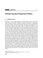
the analog domain. The magnitude response of ideal, classical analog filters are
shown in Figure 4.1. Several examples of IIR filter design are also included in
this chapter, to illustrate the design of these filters and also filters with arbitrary
magnitude response, by use of MATLAB functions. The design of FIR filters that
approximate the specifications in the frequency domain is discussed in the next
chapter.
Introduction to Digital Signal Processing and Filter Design, by B. A. Shenoi

Copyright © 2006 John Wiley & Sons, Inc.
186
INTRODUCTION
187
Magnitude
w
c
Frequency
(b)
Magnitude
w
2
w
1
Frequency
(d)
Magnitude
w
c
Frequency
(a)
Magnitude
w
1
w
2
Frequency
(c)
Figure 4.1 Magnitude responses of analog filters: (a) lowpass filter; (b) highpass filter;
(c) bandpass filter; (d) bandstop filter.

Let us select any one of the following methods to specify the IIR filters. The
recursive algorithm is given by
y(n) =−
N

k=1
a(k)y(n − k) +
M

k=0
b(k)x(n − k) (4.1)
and its equivalent form is a linear difference equation:
N

k=0
a(k)y(n − k) =
M

k=0
b(k)x(n − k); a(0) = 1 (4.2)
The transfer function of the IIR filter is given by
H(z) =

M
k=0
b(k)z
−k

N
k=0

a(k)z
−k
; a(0) = 1 (4.3)
188
INFINITE IMPULSE RESPONSE FILTERS
Let us consider a few properties of the transfer function when it is evaluated on
the unit circle z = e
jω
,whereω is the normalized frequency in radians:
H(e
jω
) =

M
k=0
b(k) cos(kω) − j

M
k=0
b(k) sin(kω)

N
k=0
a(k) cos(kω) − j

M
k=0
a(k) sin(kω)
(4.4)
=



H(e
jω
)


e
jθ(ω)
In this equation, H(e
jω
) is the frequency response, or the discrete-time Fourier
transform (DTFT) of the filter,


H(e
jω
)


is the magnitude response, and θ(e
jω
)
is the phase response. If X(e
jω
) =


X(e
jω

)


e
jα(ω)
is the frequency response of
the input signal, where


X(e
jω
)


is its magnitude and α(jω) is its phase response,
then the frequency response Y(e
jω
) is given by Y(e
jω
) = X(e
jω
)H (e
jω
) =


X(e
jω
)





H(e
jω
)


e
j {α(ω)+θ(jω)}
. Therefore the magnitude of the output signal
is multiplied by the magnitude


H(e
jω
)


and its phase is increased by the phase
θ(e
jω
) of the filter:


H(e
jω
)



=
⎧
⎪
⎨
⎪
⎩


M
k=0
b(k) cos(kω)

2
+


M
k=0
b(k) sin(kω)

2


N
k=0
a(k) cos(kω)

2
+



M
k=0
a(k) sin(kω)

2
⎫
⎪
⎬
⎪
⎭
1/2
(4.5)
θ(jω) =−tan
−1

M
k=0
b(k) sin(kω)

M
k=0
b(k) cos(kω)
+ tan
1

M
k=0
a(k) sin(kω)


N
k=0
a(k) cos(kω)
(4.6)
The magnitude squared function is


H(e
jω
)


2
=


H(e
jω
)H (e
−jω
)


=


H(e
jω
)H
∗

(e
jω
)


(4.7)
where H
∗
(e
jω
) = H(e
−jω
) is the complex conjugate of H(e
jω
). It can be shown
that the magnitude response is an even function of ω while the phase response
is an odd function of ω.
Very often it is convenient to compute and plot the log magnitude of


H(e
jω
)


as 10 log


H(e
jω

)


2
measured in decibels. Also we note that H(e
jω
)/H (e
−jω
) =
e
j2θ(ω)
. The group delay τ(jω) is defined as τ(jω) =−[dθ(jω)]/dω and is
computed from
τ(ω) =
1
1 + u
2
du
dω
−
1
1 + v
2
dv
dω
(4.8)
where
u =

M

k=0
b(k) sin(kω)

M
k=0
b(k) cos(kω)
(4.9)
MAGNITUDE APPROXIMATION OF ANALOG FILTERS
189
and
v =

N
k=0
a(k) sin(kω)

N
k=0
a(k) cos(kω)
(4.10)
Designing an IIR filter usually means that we find a transfer function H(z)
in the form of (4.3) such that its magnitude response (or the phase response, the
group delay, or both the magnitude and group delay) approximates the specified
magnitude response in terms of a certain criterion. For example, we may want
to amplify the input signal by a constant without any delay or with a constant
amount of delay. But it is easy to see that the magnitude response of a filter or
the delay is not a constant in general and that they can be approximated only by
the transfer function of the filter. In the design of digital filters (and also in the
design of analog filters), three approximation criteria are commonly used: (1) the
Butterworth approximation, (2) the minimax (equiripple or Chebyshev) approxi-

mation, and (3) the least-pth approximation or the least-squares approximation.
We will discuss them in this chapter in the same order as listed here. Designing a
digital filter also means that we obtain a circuit realization or the algorithm that
describes its performance in the time domain. This is discussed in Chapter 6. It
also means the design of the filter is implemented by different types of hardware,
and this is discussed in Chapters 7 and 8.
Two analytical methods are commonly used for the design of IIR digital fil-
ters, and they depend significantly on the approximation theory for the design
of continuous-time filters, which are also called analog filters. Therefore, it is
essential that we review the theory of magnitude approximation for analog filters
before discussing the design of IIR digital filters.
4.2 MAGNITUDE APPROXIMATION OF ANALOG FILTERS
The transfer function of an analog filter H(s) is a rational function of the complex
frequency variable s, with real coefficients and is of the form
1
H(s) =
c
0
+ c
1
s + c
2
s
2
+···+c
m
s
m
d
0

+ d
1
s + d
2
s
2
+···+d
n
s
n
,m≤ n (4.11)
The frequency response or the Fourier transform of the filter is obtained as a
function of the frequency ω,
2
by evaluating H(s) as a function of jω
H(jω) =
c
0
+ jc
1
ω − c
2
ω
2
− jc
3
ω
4
+ c
4

ω
4
+···+(j )
m
c
m
ω
m
d
0
+ jd
1
ω − d
2
ω
2
− jd
3
ω
3
+ d
4
ω
4
+···+(j )
n
c
n
ω
n

(4.12)
=
|
H(jω)
|
e
jφ(ω)
(4.13)
1
Much of the material contained in Sections 4.2–4.10 has been adapted from the author’s book
Magnitude and Delay Approximation of 1-D and 2-D Digital Filters and is included with permission
from its publisher, Springer-Verlag.
2
In Sections 4.2–4.8, discussing the theory of analog filters, we use ω and  to denote the angular
frequency in radians per second. The notation ω should not be considered as the normalized digital
frequency used in H(e
jω
).
190
INFINITE IMPULSE RESPONSE FILTERS
where H(jω) is the frequency response,
|
H(jω)
|
is the magnitude response, and
θ(jω) is the phase response. We also find the magnitude squared and the phase
response from the following:
|
H(jω)
|

2
= H(jω)H(−jω) = H(jω)H
∗
(j ω) (4.14)
H(jω)
H(−jω)
= e
j2θ(ω)
(4.15)
The magnitude response of an analog filter is an even function of ω,whereas
the phase response is an odd function. Although these properties of H(jω) are
similar to those of H(e
jω
), there are some differences. For example, the frequency
variable ω in H(jω) is (are) in radians per second, whereas ω in H(e
jω
) is
the normalized frequency in radians. The magnitude response
|
H(jω)
|
(and the
phase response) is (are) aperiodic in ω over the doubly infinite interval −∞ <
ω<∞, whereas the magnitude response


H(e
jω
)



(and the phase response) is
(are) periodic with a period of 2π on the normalized frequency scale.
Example 4.1
Let us take a simple example of a transfer function of an analog function as
H(s) =
s + 1
s
2
+ 2s + 2
(4.16)
The first step is to multiply H(s) with H(−s) and evaluate the product at
s = jω:
{
H(s)H(−s)
}|
s=jω
=
|
H(jω)
|
2
(4.17)
|
H(jω)
|
2
=
{
H(s)H(−s)

}|
s=jω
=

(s + 1)(−s + 1)
(s
2
+ s + 2)(s
2
− s + 2)





s=jω
(4.18)
=
ω
2
+ 1
ω
4
+ 1
(4.19)
From this example, we see that to find the transfer function H(s) in (4.16) from
the magnitude squared function in (4.19), we reverse the steps followed above in
deriving the function (4.19) from the H(s). In other words, we substitute jω =
s (or ω
2

=−s
2
) in the given magnitude squared function to get H(s)H(−s)
and factorize its numerator and denominator. For every pole at s
k
(and zero)
in H(s), there is a pole at −s
k
(and zero) in H(−s). So for every pole in
the left half of the s plane, there is a pole in the right half of the s plane,
and it follows that a pair of complex conjugate poles in the left half of the s
plane appear with a pair of complex conjugate poles in the right half-plane also,
thereby displaying a quadrantal symmetry. Therefore, when we have factorized
MAGNITUDE APPROXIMATION OF ANALOG FILTERS
191
the product H(s)H(−s), we pick all its poles that lie in the left half of the
s-plane and identify them as the poles of H(s), leaving their mirror images in
the right half of the s-plane as the poles of H(−s). This assures us that the
transfer function is a stable function. Similarly, we choose the zeros in the left
half-plane as the zeros of H(s), but we are free to choose the zeros in the
right half-plane as the zeros of H(s) without affecting the magnitude. It does
change the phase response of H(s), giving a non–minimum phase response.
Consider a simple example: F
1
(s) = (s + 1) and F
2
(s) = (s − 1).ThenF
22
(s) =
(s + 1)[(s − 1)/(s + 1)] has the same magnitude as the function F

2
(s) since
the magnitude of (s − 1)/(s + 1) is equal to
|
(j ω − 1)/(j ω + 1)
|
= 1forall
frequencies. But the phase of F
22
(j ω) has increased by the phase response of
the allpass function (s − 1)/(s + 1). Hence F
22
(s) is a non–minimum phase
function. In general any function that has all its zeros inside the unit circle in the
z plane is defined as a minimum phase function. If it has atleast one zero outside
the unit circle, it becomes a non–minimum phase function.
4.2.1 Maximally Flat and Butterworth Approximation
Let us choose the magnitude response of an ideal lowpass filter as shown in
Figure 4.1a. This ideal lowpass filter passes all frequencies of the input continuous-
time signal in the interval
|
ω
|
≤ ω
c
with equal gain and completely filters out all
the frequencies outside this interval. In the bandpass filter response shown in
Figure 4.1c, the frequencies between ω
1
and ω

2
and between −ω
1
and −ω
2
only
are transmitted and all other frequencies are completely filtered out.
In Figure 4.1, for the ideal lowpass filter, the magnitude response in the
interval 0 ≤ ω ≤ ω
c
is shown as a constant value normalized to one and is
zero over the interval ω
c
≤ ω<∞. Since the magnitude response is an even
function, we know the magnitude response for the interval −∞ <ω<0. For
Ideal Magnitude
Transition Band
Stopband
Passband
1.0
1 − d
p
d
s
w
p
w
s
w
Figure 4.2 Magnitude response of an ideal lowpass analog filter showing the tolerances.

192
INFINITE IMPULSE RESPONSE FILTERS
the lowpass filter, the frequency interval 0 ≤ ω ≤ ω
c
is called the passband,
and the interval ω
c
≤ ω<∞ is called the stopband. Since a transfer function
H(s) of the form (4.11) cannot provide such an ideal magnitude characteristic, it
is common practice to prescribe tolerances within which these specifications
have to be met by
|
H(jω)
|
. For example, the tolerance of δ
p
on the ideal
magnitude of one in the passband and a tolerance of δ
s
on the magnitude of
zero in the stopband are shown in Figure 4.2. A tolerance between the pass-
band and the stopband is also provided by a transition band shown in this
figure. This is typical of the magnitude response specifications for an ideal fil-
ter.
Since the magnitude squared function |H(jω)|=H(jω)H(−jω) is an even
function in ω, its numerator and denominator contain only even-degree terms;
that is, it is of the form
|
H(jω)
|

2
=
C
0
+ C
2
ω
2
+ C
4
ω
4
+···+C
2m
ω
2m
1 + D
2
ω
2
+ D
4
ω
4
+···+D
2n
ω
2n
(4.20)
In order that it approximates the magnitude of the ideal lowpass filter, let us

impose the following conditions
1. The magnitude at ω = 0 is normalized to one.
2. The magnitude monotonically decreases from this value to zero as ω →∞.
3. The maximum number of its derivatives evaluated at ω = 0 are zero.
Condition 1 is satisfied when C
0
= 1, and condition 2 is satisfied when the coeffi-
cients C
2
= C
4
= ··· =C
2m
= 0. Condition 3 is satisfied when the denominator
is 1 + D
2n
ω
2n
, in addition to condition 2 being satisfied. The magnitude response
that satisfies conditions 2 and 3 is known as the Butterworth response,whereas
the response that satisfies only condition 3 is known as the maximally flat mag-
nitude response, which may not be monotonically decreasing. The magnitude
squared function satisfying the three conditions is therefore of the form
|
H(jω)
|
2
=
1
1 + D

2n
ω
2n
(4.21)
We scale the frequency ω by ω
p
and define the normalized analog frequency
 = ω/ω
p
so that the passband of this filter is 
p
= 1. Now the magnitude of
the lowpass filter satisfies the three conditions listed above and also the condition
that its passband be normalized to 
p
= 1. Such a filter is called a prototype
lowpass Butterworth filter having a transfer function H(p) = H(s/p),which
has its magnitude squared function given by
|
H(j)
|
2
=
1
1 + D
2n

2n
(4.22)
The following specifications are normally given for a lowpass Butterworth filter:

(1) a magnitude of H
0
at ω = 0, (2) the bandwidth ω
p
, (3) the magnitude at the
MAGNITUDE APPROXIMATION OF ANALOG FILTERS
193
bandwidth ω
p
, (4) a stopband frequency ω
s
, and (5) the magnitude of the filter
at ω
s
. The transfer function of the analog filter with practical specifications like
these will be denoted by H(p) in the following discussion, and the prototype
lowpass filter will be denoted by H(s).
Before we proceed with the analytical design procedure, we normalize the
magnitude of the filter by H
0
for convenience and scale the frequencies ω
p
and
ω
s
by ω
p
so that the bandwidth of the prototype filter and its stopband fre-
quency become 
p

= 1and
s
= ω
s
/ω
p
, respectively. The specifications about
the magnitude at 
p
and 
s
are satisfied by the proper choice of D
2n
and n
in the function (4.22) as explained below. If, for example, the magnitude at the
passband frequency is required to be 1/
√
2, which means that the log magnitude
required is −3 dB, then we choose D
2n
= 1. If the magnitude at the passband
frequency  = 
p
= 1 is required to be 1 − δ
p
, then we choose D
2n
, normally
denoted by 
2

, such that
|
H(j1)
|
2
=
1
1 + D
2n
=
1
1 + 
2
= (1 − δ
p
)
2
(4.23)
If the magnitude at the bandwidth  = 
p
= 1 is given as −A
p
decibels, the
value of 
2
is computed by
10 log
1
1 + 
2

=−A
p
10 log(1 + 
2
) = A
p
log(1 + 
2
) = 0.1A
p
(1 + 
2
) = 10
0.1A
p
From the last equation, we get the formula 
2
= 10
0.1A
p
− 1and =

10
0.1A
p
− 1.
Let us consider the common case of a Butterworth filter with a log magnitude
of −3 dB at the bandwidth of 
p
to develop the design procedure for a Butter-

worth lowpass filter. In this case, we use the function for the prototype filter, in
the form
|
H(j)
|
2
=
1
1 + 
2n
(4.24)
This satisfies the following properties:
1. The magnitude squared of the filter response at  = 0 is one.
2. The magnitude squared at  = 1is
1
2
for all integer values of n;sothelog
magnitude is −3dB.
3. The magnitude decreases monotonically to zero as  →∞; the asymptotic
rate is −40n dB/decade.
194
INFINITE IMPULSE RESPONSE FILTERS
1.2
1
0.8
0.6
0.4
0.2
0
Magnitude

0
0.5
1
1.5
2
2.5
3
3.5
4
Frequency in rad/sec
n = 2
n = 6
Figure 4.3 Magnitude responses of Butterworth lowpass filters.
The magnitude response of Butterworth lowpass filters is shown for n =
2, 3,...,6 in Figure 4.3. Instead of showing the log magnitude of these filters,
we show their attenuation in decibels in Figure 4.4. Attenuation or loss measured
in decibels is defined as
−10 log
|
H(j)
|
2
= 10 log(1 + 
2n
)
The attenuation over the passband only is shown in Figure 4.4a, and the maximum
attenuation in the passband is 3 dB for all n; the attenuation characteristic of the
filters over 1 ≤  ≤ 10 for n = 1, 2,...,10 is shown in Figure 4.4b.
4.2.2 Design Theory of Butterworth Lowpass Filters
Let us consider the design of a Butterworth lowpass filter for which (1) the

frequency ω
p
at which the magnitude is 3 dB below the maximum value at ω = 0,
and (2) the magnitude at another frequency ω
s
in the stopband are specified.
When we normalize the gain constant to unity and normalize the frequency by
the scale factor ω
p
, we get the cutoff frequency of the normalized prototype
filter 
p
= 1 and the stopband frequency 
s
= ω
s
/ω
p
. After we have found the
transfer function H(p) of this normalized prototype lowpass filter, we restore
the frequency scale and the magnitude scale to get the transfer function H(s)
approximating the prescribed magnitude specification of the lowpass filter.
The analytical procedure used to derive H(p) from the magnitude squared
function of the prototype lowpass filter is carried out simply by reversing the
MAGNITUDE APPROXIMATION OF ANALOG FILTERS
195
7.0
6.0
4.0
5.0

1.0
3.0
2.0
0
0 0.2
0.4 0.6
0.8 1.0
n = 1
2
6
5
4
3
7
8
9
10
Passband attenuation a, dB
(a)
ω
ω
10
9
8
7
6
5
4
3
2

n = 1
140
120
100
80
60
40
20
0
Stopband attenuation a, dB
0 2.0 4.0 6.0 8.0 10
(b)
Figure 4.4 Attenuation characteristics of Butterworth lowpass filters in (a) passband;
(b) stopband.
196
INFINITE IMPULSE RESPONSE FILTERS
steps used to derive the magnitude squared function from H(p) as illustrated by
Example 4.1 earlier. First we substitute  = p/j or equivalently 
2
=−p
2
in
(4.24):
1
1 + 
2n






2
=−p
2
=
1
1 + (−1)
n
p
2n
= H(p)H(−p) (4.25)
The denominator has 2n zeros obtained by solving the equation
1 + (−)
n
p
2n
= 0 (4.26)
or the equation
p
2n
=

1 = e
j2kπ
n odd
−1 = e
j(2k+1)π
n even
(4.27)
This gives us the 2n poles of H(p)H(−p), which are

p
k
= e
j(2kπ/2n)π
k = 1, 2,...,(2n) when n is odd (4.28)
and
p
k
= e
j[(2k−1)/2n]π
k = 1, 2,...,(2n) when n is even (4.29)
or in general
p
k
= e
j[(2k+n−1)/2n]π
k = 1, 2,...,(2n) (4.30)
We notice that in both cases, the poles have a magnitude of one and the angle
between any two adjacent poles as we go around the unit circle is equal to π/n.
There are n poles in the left half of the p plane and n poles in the right half of
the p plane, as illustrated for the cases of n = 2andn = 3 in Figure 4.5. For
every pole of H(p) at p = p
a
that lies in the left half-plane, there is a pole of
H(−p) at p =−p
a
that lies in the right half-plane. Because of this property,
we identify n poles that are in the left half of the p plane as the poles of H(p)
so that it is a stable transfer function; the poles that are in the right half-plane
are assigned as the poles of H(−p).Then poles that are in the left half of the

p plane are given by
p
k
= exp

j

2k + n − 1
2n

π

k = 1, 2, 3,...,n (4.31)
When we have found these n poles, we construct the denominator polynomial
D(p) of the prototype filter H(p) =
1
D(p)
from
D(p) =
n

k=1
(p − p
k
) (4.32)
MAGNITUDE APPROXIMATION OF ANALOG FILTERS
197
π
2
n = 2

π
3
q
1
q
2
q
3
n = 3
Figure 4.5 Pole locations of Butterworth lowpass filters of orders n = 2andn = 3.
The only unknown parameter at this stage of design is the order n of the filter
function H(p), which is required in (4.31). This is calculated using the specifi-
cation that at the stopband frequency 
s
, the log magnitude is required to be no
more than −A
s
dB or the minimum attenuation in the stopband to be A
s
dB.
10 log
|
H(j
s
)
|
2
=−10 log(1 + 
2n
s

) ≤−A
s
(4.33)
from which we derive the formula for calculating n as follows:
n ≥
log(10
0.1A
s
− 1)
2log
s
(4.34)
Since we require that n be an integer, we choose the actual value of n =n
that is the next-higher integer value or the ceiling of n obtained from the right
side of (4.34). When we choose n =n, the attenuation in the stopband is more
than the specified value of A
s
. We use this integer value for n in (4.31), to cal-
culate the poles and then construct the denominator polynomial D(p) of order
n. By multiplying (p − p
k
) with (p − p
∗
k
) where p
k
and p
∗
k
are complex con-

jugate pairs, the polynomial is reduced to the normal form with real coefficients
only. These polynomials, known as Butterworth polynomials, have many special
properties. In the polynomial form, if we represent them as
D(p) = 1 + d
1
p + d
2
p
2
+···+d
n
p
n
(4.35)
their coefficients can be computed recursively from (d
0
= 1)
d
k
=
cos

(k − 1)
π
2

sin

kπ
2n

 d
k−1
k = 1, 2, 3,...,n (4.36)
But there is no need to do so, since they can be computed from (4.32). They are
also listed in many books for n up to 10 in polynomial form and in some books
in a factored form also [3,2]. We list a few of them in Table 4.1.
198
INFINITE IMPULSE RESPONSE FILTERS
TABLE 4.1
n Butterworth Polynomial D(p) in Polynomial and Factored Form
1 p + 1
2 p
2
+
√
2p + 1
3 p
3
+ 2p
2
+ 2p + 1 = (p + 1)(p
2
+ p + 1)
4 p
4
+ 2.61326p
3
+ 3.41421p
2
+ 2.61326p + 1

= (p
2
+ 0.76537p + 1)(p
2
+ 1.84776p + 1)
5 p
5
+ 3.23607p
4
+ 5.23607p
3
+ 5.23607p
2
+ 3.23607p + 1
= (p + 1)(p
2
+ 0.618034p + 1)(p
2
+ 1.931804p + 1)
6 p
6
+ 3.8637p
5
+ 7.4641p
4
+ 9.1416p
3
+ 7.4641p
2
+ 3.8637p + 1

= (p
2
+ 0.5176p + 1)(p
2
+ 1.4142p + 1)(p
2
+ 1.9318p + 1)
In the case of lowpass filters, usually the magnitude is specified at ω = 0;
hence it is also the magnitude at  = 0. Therefore the specified magnitude is
equated to the value of the transfer function H(p) evaluated at p = j0. This is
equal to H(j0) = H
0
/D(j 0) = H
0
. So we restore the magnitude scale by mul-
tiplying the normalized prototype filter function by H
0
. To restore the frequency
scale by ω
p
, we put p = s/ω
p
in H
0
/D(p) and simplify the expression to get
transfer function H(s) for the specified lowpass filter. This completes the design
procedure, which will be illustrated in Example 4.2.
Example 4.2
Design a lowpass Butterworth filter with a maximum gain of 5 dB and a cutoff
frequency of 1000 rad/s at which the gain is at least 2 dB and a stopband fre-

quency of 5000 rad/s at which the magnitude is required to be less than −25 dB.
The maximum gain of 5 dB is the magnitude of the filter function at ω = 0.
The edge of the passband is the cutoff frequency ω
p
= 1000, and the frequency
range 0 ≤ ω ≤ ω
p
is called the bandwidth. So we see that the magnitude of
2 dB at this frequency is 3 dB below the maximum value in the passband. We
say that the filter has a 3 dB bandwidth equal to 1000 rad/s. The frequency scale
factor is chosen as 1000 so that the passband of the prototype filter is 
p
= 1.
The stopband frequency ω
s
is specified as 5000 rad/s and is therefore scaled to

s
= 5. The magnitude is normalized so that the normalized prototype lowpass
filter function H(p)
3
has a magnitude of one (i.e., 0 dB) at  = 0. It is this filter
that has a magnitude squared function
|
H(j)
|
2
=
1
1 + 

2n
(4.37)
3
Note that we have chosen p =

+j as the notation for the complex frequency variable of the
transfer function H(p) for the lowpass prototype filter and the notation s = σ + jω for the variable
of the transfer function H(s) for the specified filter.
MAGNITUDE APPROXIMATION OF ANALOG FILTERS
199
(a)
0 dB
−3
−30
Magnitude in dB
w
(b)
0 dB
−0.5
−30
Magnitude in dB
w
Figure 4.6 Magnitude response specifications of prototype filters: (a) Butterworth filter;
(b) Chebyshev (equiripple) filter.
It is always necessary to reduce the given specifications to the specifications of
this normalized prototype filter to which only the expressions derived above are
applicable. The magnitude response of the normalized prototype filter (not to
scale) for this example is shown in Figure 4.6a.
For this example, note that the maximum attenuation in the passband is A
p

=
3 dB and the minimum attenuation in the stopband is A
s
= 30 dB. From (4.34)
we calculate the value of n = 2.1457 and choose n =2.1457=3. From (4.31),
we get the three poles as p
1
=−0.5 + j
√
0.75, p
2
=−1.0andp
3
=−0.5 −
j
√
0.75. Therefore the third-order denominator polynomial D(p) is obtained
from (4.32) or from Table 4.1:
D(p) = (p + 0.5 − j
√
0.75)(p + 1)(p + 0.5 +

0.75)
= (p
2
+ p + 1)(p + 1) = p
3
+ 2p
2
+ 2p + 1 (4.38)

Hence the transfer function of the normalized prototype filter of third order is
H(p)=
1
p
3
+ 2p
2
+ 2p + 1
(4.39)
To restore the magnitude scale, we multiply this function by H
0
. Now the filter
function is
H(p)=
H
0
p
3
+ 2p
2
+ 2p + 1
(4.40)
which has a magnitude of H
0
at p = j0. From the requirement 20 log(H
0
) =
5 dB, we calculate the value of H
0
= 1.7783. To restore the frequency scale, we

200
INFINITE IMPULSE RESPONSE FILTERS
substitute p = s/1000 in (4.40) and simplify to get H(s) as shown below:
H(p)
|
p=s/1000
=
1.7783

s
1000

3
+ 2

s
1000

2
+ 2

s
1000

+ 1
=
(1.7783)10
9
s
3

+ (2 × 10
3
)s
2
+ (2 × 10
6
)s + 10
9
(4.41)
= H(s) (4.42)
The magnitude of H(p) plotted on the normalized frequency scale  shown in
Figure 4.7 is marked as “Example (2).” It is found that the attenuation at the
stopband edge 
s
= 5 is about 42 dB, which is more than the specified 30 dB.
It must be remembered that in (4.37) 
p
= 1 is the bandwidth of the prototype
filter, and at this frequency,
|
H(j)
|
2
has a value of
1
2
or a magnitude of −3dB.
Hence formulas (4.31) and (4.34) cannot be used if the maximum attenuation A
p
in the passband is different from 3 dB. In this case, we modify the function to

the form (4.43), which is the general case:
|
H(j)
|
2
=
1
1 + 
2

2n
(4.43)
Now the attenuation at  = 1 is given by 10 log(1 + 
2
) = A
p
, from which we
get 
2
= (10
0.1A
p
− 1). We may also note that 
2
= 1 in the previous case when
A
p
= 3. When A
p
is other than 3 dB, the formulas for calculating n and p

k
are
n ≥
log

(10
0.1A
s
− 1)/(10
0.1A
p
− 1)

2log
s
(4.44)
Example (3)
Example (4)
Example (2)
Fre
q
uenc
y
in radians/sec-linear scale
10
°
Magnitude in dB
0
−1
−2

−
3
−
4
−
5
Figure 4.7 Magnitude responses of the prototype filters in Examples 4.1–4.3.
MAGNITUDE APPROXIMATION OF ANALOG FILTERS
201
and
p
k
= 
−(1/n)
exp

j

2k + n − 1
2n

π

k = 1, 2, 3,...,n (4.45)
Comparing (4.45) with (4.31), it is obvious that the poles have been scaled by a
factor 
−(1/n)
. So the maximum attenuation at 
p
= 1 is the specified value of

A
p
; also the frequency at which the attenuation is 3 dB is equal to 
−(1/n)
.
Example 4.3
Design a lowpass Butterworth filter with a maximum magnitude of 5 dB, pass-
band of 1000 rad/s, maximum attenuation in the passband A
p
= 0.5dB, and
minimum attenuation A
s
= 30 dB at the stopband frequency of 5000 rad/s.
First we scale the frequency by ω
p
= 1000 so that the normalized passband
frequency 
p
= 1 and the stopband frequency ω
s
is mapped to 
s
= 5. Also
the magnitude is scaled by 5 dB. The magnitude response for the normalized
prototype filter H(p) is similar to that shown in Figure 4.6a, except that now
A
p
= 0.5 dB. Then we calculate 
2
= (10

0.1A
p
− 1) = 0.1220 and therefore  =
0.3493. From (4.44), the value of n = 2.7993; it is rounded to n=3. Next we
compute the three poles from (4.45) as p
1
=−0.71 + j1.2297, p
2
=−1.4199,
and p
3
=−0.71 − j1.2297. The transfer function of the filter with these poles is
H(p)=
H
0
(p + 1.4199)(p + 0.71− j1.2297)(p + 0.71 + j1.2297)
=
H
0
(p + 1.4199)(p
2
+ 1.42p + 2.0163)
(4.46)
Since the maximum value has been normalized to 0 dB, which occurs at  = 0,
we equate the magnitude of H(p) evaluated at p = j0 to one. Therefore H
0
=
(1.4199)(2.0163) = 2.8629. To raise the magnitude level to 5 dB, we have to
multiply this constant by
√

10
0.5
= 1.7783. Of course, we can compute the same
value for H
0
in one step, from the specification 20 log
|
H(j0)
|
= 20 log H(0) −
20 log(1.4199)(2.0163) = 5. The frequency scale is restored by putting p =
s/1000 in (4.46) to get (4.47) as the transfer function of the filter that meets
the given specifications:
H(s)=
(2.8629)(1.7783)
[s/1000 + 1.4199][(s/1000)
2
+ 1.42(s/1000) + 2.0163]
=
5.09 × 10
9
[s + 1419.9][s
2
+ 1420s + 2.0163 × 10
6
]
(4.47)
The plot is marked as “Example (3)” in Figure 4.7. It is the magnitude response
of the prototype filter given by (4.46). It has a magnitude of −0.5 dB at  = 1
and approximately −33 dB at  = 5, which exceeds the specified value.

202
INFINITE IMPULSE RESPONSE FILTERS
4.2.3 Chebyshev I Approximation
The Chebyshev I approximation for an ideal lowpass filter shows a magnitude
that has the same values for the maxima and for the minima in the passband and
decreases monotonically as the frequency increases above the cutoff frequency.
It has equal-valued ripples in the passband between the maximum and minimum
values as shown in Figure 4.6b. Hence it is known as the minimax approximation
and also as the equiripple approximation. To approximate the ideal magnitude
response of the lowpass filter in the equiripple sense, the magnitude squared
function of its prototype is chosen to be
|
H(j)
|
2
=
H
2
0
1 + 
2
C
2
n
()
(4.48)
where C
n
() is the Chebyshev polynomial of degree n.Itisdefinedby
C

n
() = cos(n cos
−1
)
|

|
≤ 1 (4.49)
The polynomial C
n
() approximates a value of zero over the closed interval
 ∈ [−1, 1] in the equiripple sense as shown by examples for n = 2, 3, 4, 5
in Figure 4.8a. These polynomials are
C
0
() = 1
C
1
() = 
C
2
() = 2
2
− 1
C
3
() = 4
3
− 3
C

4
() = 8
4
− 8
2
+ 1
C
5
() = 16
5
− 20
3
+ 5 (4.50)
4.2.4 Properties of Chebyshev Polynomials
Some of the properties of Chebyshev polynomials that are useful for our discus-
sion are described below. Let cos φ = .ThenC
n
(n cos
−1
) = cos(nφ),and
therefore we use the identity
cos(k + 1) = cos(kφ) cos(φ) − sin(kφ) sin(φ)
= 2cos(kφ) cos(φ) − cos((k − 1)φ) (4.51)
from which we obtain a recursive formula to generate Chebyshev polynomials
of any order, as
C
0
() = 1
C
k+1

() = 2C
k
() − C
k−1
() (4.52)
MAGNITUDE APPROXIMATION OF ANALOG FILTERS
203
(a)
(b)
C
2
(Ω)
C
4
(Ω)
C
3
(Ω)
1
1
1
1
1
1
C
5
(Ω)
1
1
10log(l + e

2
C
4
2
(Ω))
Ω
p
= 1
A
p
Figure 4.8 Chebyshev polynomials and Chebyshev filter: (a) magnitude of Chebyshev
polynomials; (b) attenuation of a Chebyshev I filter.
To see that C
n
() = cos(n cos
−1
) is indeed a polynomial of order n, consider
it in the following form:
cos(nφ) = Re

e
jnφ

= Re

cos(φ) + j sin(φ

n
= Re


φ + j

(1 − φ
2

n
= Re

φ +

φ
2
− 1

n
(4.53)
Expanding

φ +

φ
2
− 1

n
by the binomial theorem and choosing the real part,
we get the polynomial for
cos(nφ) = φ
n
+

n(n − 1)
2!
φ
n−2
(φ
2
− 1)
+
n(n − 1)(n − 2)(n − 3)
4!
φ
n−4
(φ
2
− 1)
2
+··· (4.54)
204
INFINITE IMPULSE RESPONSE FILTERS
Recall that since n is a positive integer, the expansion expressed above has a
finite number of terms, and hence we conclude that it is a polynomial (of degree
n). We also note from (4.50) that
C
2
n
(0) =

0 n odd
1 n even
(4.55)

But
C
2
n
(1) =

1 n odd
1 n even
(4.56)
So we derive the following properties:
|
H(0)
|
2
=

1 n odd
1
1+
2
n even
(4.57)
|
H(1)
|
2
=
1
1 + 
2

n odd or even (4.58)
The attenuation characteristics of the Chebyshev filter of order n = 4 is shown in
Figure 4.8b as an example. The magnitude
|
H(j)
|
plotted as “Example(4)” in
Figure 4.7 has an equiripple response in the passband, with a maximum value of
0 dB and a minimum value of 10 log[1/(1 + 
2
)] decibels. However, the mag-
nitude of Chebyshev I lowpass filters is 10 log[1/(1 + 
2
)]at = 1forany
order n. The magnitude of the ripple can be measured as either
|
H(0)
|
−
|
H(1)
|
or
|
H(0)
|
2
−
|
H(1)

|
2
= 1 − [1/(1 + 
2
)] = [
2
/(1 + 
2
)] ≈ 
2
.Wecanalways
calculate 
2
= (10
0.1A
p
− 1).
Another property of Chebyshev I filters is that the total number of maxima and
minima in the closed interval [−11]isn + 1. The square of the magnitude
response of Chebyshev lowpass filters is shown in Figure 4.9a to indicate some
properties of the Chebyshev lowpass filters just described.
4.2.5 Design Theory of Chebyshev I Lowpass Filters
Typically the specifications for a lowpass Chebyshev filter specify the maximum
and minimum values of the magnitude in the passband; the cutoff frequency ω
p
,
which is the highest frequency of the passband; a frequency ω
s
in the stopband;
and the magnitude at the frequency ω

s
. As in the case of the Butterworth filter, we
normalize the magnitude and the frequency and reduce the given specifications
to those of the normalized prototype lowpass filter and follow similar steps to
find the poles of H(p).
Since  can take real values greater than one in general, let us assume φ to be
a complex variable: φ = ϕ
1
+ jϕ
2
.From1+ 
2
C
2
n
() = 0, we get 
2
C
2
n
() =
MAGNITUDE APPROXIMATION OF ANALOG FILTERS
205
n = 3 (odd)
Ω
p
Ω
s
⏐H( jΩ)⏐
2

1
n = 4 (even)
Ω
p
Ω
s
⏐H( jΩ)⏐
2
1
n = 4 (even)
Ω
p
Ω
s
⏐H( jΩ)⏐
2
1
n = 5 (odd)
Ω
p
Ω
s
⏐H( jΩ)⏐
2
1
(a)
(b)
Figure 4.9 Magnitude response of Chebyshev filters: (a) Chebyshev I filters;
(b) Chebyshev II filters.
−1 = j

2
;wederive
C
n
() =±
j

= cos(nφ) = cos(n(ϕ
1
+ jϕ
2
))
= cos(nϕ
1
) cosh(nϕ
2
) − j sin(nϕ
1
) sin(nϕ
2
) (4.59)
Equating the real and imaginary parts, we get
cos(nϕ
1
) cosh(nϕ
2
) = 0 (4.60)
and
sin(nϕ
1

) sin(nϕ
2
) =∓
1

(4.61)
From (4.60) we get
ϕ
1
=
(2k − 1)π
2n
(4.62)
206
INFINITE IMPULSE RESPONSE FILTERS
Substituting this in (4.61), we obtain sinh(nϕ
2
) =±(1/), from which we get
ϕ
2
=
1
n
sinh
−1

1


(4.63)

Now  = cos(φ) = cos(ϕ
1
+ jϕ
2
) = cos(ϕ
1
) cosh(ϕ
2
) − j sin(ϕ
1
) sinh(ϕ
2
).
Therefore
j = sin(ϕ
1
) sinh(ϕ
2
) + j cos(ϕ
1
) cosh(ϕ
2
) (4.64)
These are the roots in the p plane that satisfy the condition 1 + 
2
C
2
n
() = 0.
Hence the 2n poles of H(p)H(−p) are given by

p
k
= sinh(ϕ
2
) sin

(2k − 1)π
2n

+ j cosh(ϕ
2
) cos

(2k − 1)π
2n

for
k = 1, 2,...,(2n) (4.65)
The 2n poles of H(p)H(−p) given by (4.65) can be shown to lie on an elliptic
contour in the p plane with a major semiaxis equal to cosh(ϕ
2
) along the j
axis and a minor semiaxis equal to sinh(ϕ
2
) along  axis, where p =

+j.
We find that the frequency 
3
at which the attenuation of the prototype filter is

3dBisgivenby

3
= cosh

1
n
cosh
−1

1


(4.66)
The poles in the left half of the p plane only are given by
p
k
=−sinh(ϕ
2
) sin

(2k − 1)π
2n

+ j cosh(ϕ
2
) cos

(2k − 1)π
2n


=−sinh(ϕ
2
) sin(θ
k
) + j cosh(ϕ
2
) cos(θ
k
)k= 1, 2, 3,...,n (4.67)
where ϕ
2
is obtained from (4.63). In (4.67), note that θ
k
are the angles measured
from the imaginary axis of the p plane and the poles lie in the left half of the
p plane.
The formula for finding the order n is derived from the requirement that
10 log[1 + 
2
C
2
n
(
s
)] ≥ A
s
.Itis
n ≥
cosh

−1


(10
0.1A
s
− 1)/(10
0.1A
p
− 1)

cosh
−1

s
(4.68)
and the value of n is chosen for calculating the poles using (4.67). Given ω
p
,
A
p
, ω
s
,andA
s
as the specifications for a Chebyshev lowpass filter H(s), its
MAGNITUDE APPROXIMATION OF ANALOG FILTERS
207
maximum value in the passband is normalized to one, and its frequencies are
scaled by ω

p
, to get the values of 
p
= 1and
s
= ω
s
/ω
p
for the prototype
filter at which the attenuations are A
p
and A
s
, respectively. The design procedure
to find H(s) starts with the magnitude squared function (4.48) and proceeds as
follows:
1. Calculate  =

(10
0.1A
p
− 1).
2. Calculate n from (4.68) and choose n =n.
3. Calculate ϕ
2
from (4.63).
4. Calculate the poles p
k
(k = 1, 2,...,n) from (4.67).

5. Compute H(p) = H
0
/[

n
k=1
(p − p
k
)] = H
0
/[

n
k=0
d
k
p
k
].
6. Find the value of H
0
by equating
H(0) =
H
0
d
0
=
⎧
⎨

⎩
1 n odd

1
1 + 
2
n even
7. Restore the magnitude scale.
8. Restore the frequency scale by substituting p = s/ω
p
in H(p) and simplify
to get H(s).
A simple example is worked out below to illustrate this design procedure.
Example 4.4
Let us choose the specifications of a lowpass Chebyshev filter with a maxi-
mum gain of 5 dB, a bandwidth of 2500 rad/s, and a stopband frequency of
12,500 rad/s; A
p
= 0.5dB,andA
s
= 30 dB. For the prototype filter, the maxi-
mum value in the passband is one (0 dB), and we have 
p
= 1, 
s
= 5. So
1.  =

(10
0.05

− 1 = 0.34931.
2. n ≥{cosh
−1


(10
3
− 1)/(10
0.05
− 1)

}/[cosh
−1
(5)] = 2.2676; choose
n = 3.
3. ϕ
2
=
1
3
sinh
−1

1
0.34931

= 0.591378.
4. p
k
=−0.313228 ± j1.02192 and −0.626456.

5. H(p) = H
0
/[(p + 0.31228 − j1.02192)(p + 0.31228 + j 1.02192)(p +
0.626456)] = H
0
/[(p
2
+ 0.626456p + 1.142447)(p + 0.626456)].
6. H(0) = H
0
/[(1.142447)(0.626456)] = 1(sincen = 3 is odd). Hence H
0
=
0.715693.
7. The transfer function with a direct-current (DC) gain of 0 dB is H(p) =
0.715693/[(p
2
+ 0.626456p + 1.142447)(p + 0.626456)]. The magnitude
scale is restored by multiplying H(p) by 1.7783, so that the DC gain is
raised to 5 dB.
208
INFINITE IMPULSE RESPONSE FILTERS
8. The transfer function of the filter is
H(p) =
(0.715693)(1.7783)
(p
2
+ 0.626456p + 1.142447)(p + 0.626456)
(4.69)
When we substitute p = s/2500 in this H(p) and simplify the expression, we get

H(s) =
19.886 × 10
12
(s
2
+ 1566s + 714 × 10
6
)(s + 1566)
(4.70)
The magnitude response of the prototype filter in (4.70) is marked as “Example(4)”
in Figure 4.7. The three magnitude responses are plotted in the same figure so
that the response of the three filters can be compared. The attenuation of the
Chebyshev filter at 
s
= 5 is found to be 47 dB. The abovementioned class of
filters with equiripple passband response and monotonic response in the stopband
are sometimes called Chebyshev I filters, to distinguish them from the following
class of filters, known as Chebyshev II filters.
4.2.6 Chebyshev II Approximation
The Chebyshev II filters have a magnitude response that is maximally flat at ω =
0; it decreases monotonically as the frequency increases and has an equiripple
response in the stopband. Typical magnitudes of Chebyshev II filters are shown
in Figure 4.9b. This class of filters are also called Inverse Chebyshev filters.The
transfer function of Chebyshev II filters are derived by applying the following
two transformations: (1) a frequency transformation  = 1/ω in
|
H(j)
|
2
of

the lowpass normalized prototype filter gives the magnitude squared function of
the highpass filter
|
H(1/j )
|
2
, with an equiripple passband in
|

|
> 1anda
monotonically decreasing response in the stopband 0 <
|

|
< 1; (2) when it is
subtracted from one, we get the magnitude squared function (4.72) of the inverse
Chebyshev lowpass filter:




H
1
j




2

=
1
1 + 
2
C
2
n
(1/)
(4.71)
1 −
1
1 + 
2
C
2
n
(1/)
=

2
C
2
n
(1/)
1 + 
2
C
2
n
(1/)

=
1

1 +
1

2
C
2
n
(1/)

(4.72)
The magnitude squared function |H(j)|
2
of a lowpass Chebyshev I filter
and |H(
1
j
)|
2
and 1 −|H(
1
j
)|
2
are shown in Figure 4.10.
We make two important observations in Figure 4.10. The normalized cutoff
frequency  = 1 becomes the lowest frequency in the stopband of the inverse
Chebyshev filter at which the magnitude is 

2
/(1 + 
2
). Hence the frequencies ω
p
and ω
s
specified for the inverse Chebyshev filter must be scaled by ω
s
and not by
ω
p
to obtain the prototype of the inverse Chebyshev filter. We also observe that
MAGNITUDE APPROXIMATION OF ANALOG FILTERS
209
Ω
Ω
Ω
H(jΩ)
1
H(
2
1
jΩ
)
1−
||
H(
2
1

jΩ
)
||
2
||
Figure 4.10 Transformation of Chebyshev I–Chebyshev II filter response.
when n is odd, the number of finite zeros in the stopband is (n − 1)/2 = m.When
n is an odd integer, the term sec θ
k
, which is involved in the design procedure
described below, attains a value of ∞ when k = (n + 1)/2. So one of the zeros
is shifted to j ∞; the remaining finite zeros appear in conjugate pairs on the
imaginary axis, and hence the numerator of the Chebyshev II filter is expressed
as shown in step 6 in Section 4.2.7. Note that the value of 
i
calculated in step 1
is different from the value calculated in the design of Chebyshev I filters and
therefore the values of ϕ
i
used in steps 3 and 4 are different from ϕ
2
used in
the design of Chebyshev I filters. Hence it would be misleading to state that the
poles of the Chebyshev II filters are obtained as “the reciprocals of the poles of
the Chebyshev I filters.”
210
INFINITE IMPULSE RESPONSE FILTERS
4.2.7 Design of Chebyshev II Lowpass Filters
Given ω
p

, A
p
, ω
s
, A
s
and the maximum value in the passband, we scale the
frequencies ω
p
and ω
s
by ω
s
and deduce the specifications for the normalized
prototype lowpass inverse Chebyshev filter. Equation (4.72) is the magnitude
squared function of this inverse Chebyshev filter, and we follow the design pro-
cedure as outlined below:
1. Calculate 
i
= 1/

(10
0.1A
s
− 1).
2. Calculate
n ≥
cosh
−1



(10
0.1A
s
− 1)/(10
0.1A
p
− 1)

cosh
−1

s
and choose n =n.
3. Calculate ϕ
i
from ϕ
i
= (1/n) sinh
−1
(1/
i
).
4. Compute the poles in the left-half plane p
k
:
p
k
=
1

− sinh(ϕ
i
) sin(θ
k
) + j cosh(ϕ
i
) cos(θ
k
)
k = 1, 2, 3,...,n
5. The zeros of the transfer function H(p) are calculated as z
k
=±j
0k
=
j sec θ
k
for k = 1, 2,...,m=n/2 and the numerator N(p) of H(p) as

m
k=1
(p + 
2
ok
)
6. Compute
H(p)=
H
0


m
k=1
(p + 
2
0k
)

n
k=1
(p − p
k
)
and calculate H
0
=

n
k=1
(p
k
)/

m
k=1
(
0k
)
2
.
7. Restore the magnitude scale.

8. Restore the frequency scale by putting p = s/ω
s
in H(p) to get H(s) for
the inverse Chebyshev filter.
Example 4.5
Design the lowpass inverse Chebyshev filter with a maximum gain of 0 dB
in the passband, ω
p
= 1000, A
p
= 0.5dB, ω
s
= 2000, and A
s
= 40 dB. We
normalize the frequencies by ω
s
and get the lowest frequency of the stopband
at  = 1, while ω
p
= 1000 maps to 
p
= 0.5. We will have to denormalize the
frequency by substituting p = s/2000 when the transfer function H(p) of the
inverse Chebyshev filter, obtained by the steps given above, is completed. The
design procedure gives
1. 
i
= (
√

10
4
− 1)
−1
=
1
99.995
.
2. n = 5.