A memetic algorithm for the integral OBP/OPP problem in a logistics distribution center
Bạn đang xem bản rút gọn của tài liệu. Xem và tải ngay bản đầy đủ của tài liệu tại đây (380.4 KB, 12 trang )
Uncertain Supply Chain Management 7 (2019) 203–214
Contents lists available at GrowingScience
Uncertain Supply Chain Management
homepage: www.GrowingScience.com/uscm
A memetic algorithm for the integral OBP/OPP problem in a logistics distribution center
Fabio Miguela, Mariano Frutosb*, Fernando Tohméc and Daniel A. Rossitb
a
Sede Alto Valle y Valle Medio, Universidad Nacional de Río Negro. Villa Regina, Argentina
Department of Engineering, Universidad Nacional del Sur and IIESS-CONICET. Bahía Blanca, Argentina
c
Department of Economics, Universidad Nacional del Sur and INMABB-CONICET. Bahía Blanca, Argentina
b
CHRONICLE
Article history:
Received September 9, 2018
Accepted October 12 2018
Available online
October 12 2018
Keywords:
Order Batching Problem
Order Picking Problem
Optimization
Logistics
ABSTRACT
In this paper, we present a new decision-making tool aimed at improving the efficiency of the
operational planning of pick-up processes in logistic distribution centers. It is based on a memetic
algorithm (MA) solving both the Order Batching Problem (OBP) and the Order Picking Problem
(OPP). The result yields a sequence of simultaneous pick up operations of lots for different
clients in a storing facility, satisfying a previously defined distribution plan. The objective is the
minimization of the operational cost of the entire process, which is directly proportional to the
time spent on different activities involved. The failure to satisfy the conditions, either leads to
overstocking, delays in delivery or creates inefficiency costs. The analysis of the results obtained
with our algorithmic tool indicates that it has a good performance in comparison with other
known algorithms used to solve this kind of problem.
© 2019 by the authors; licensee Growing Science, Canada
1. Introduction
The optimization of processes in a distribution center is a critical factor for the operational performance
of the internal and external logistics of the firm. These operational processes, as for instance reception,
placement, storing, selection, order picking, classification and dispatch, involve moving goods inside
distribution centers (Biswas & Das, 2018).
Depots or storage sites play different roles according to the logistic system in which they are used.
This, in turn, has consequences for the optimal use of those spaces. One of these roles is crucial in
extended or permanent storage systems, i.e. systems in which the records of activity of products indicate
frequencies of access to long-term storage positions. The main goal of the optimization of processes in
this kind of system is the efficient use of space while optimal speed of access and flow of materials is
not a priority. A different kind of storage site is used in active storage systems, whose main function is
not to store wares for long periods of time but to facilitate the distribution of goods. Here the goal is
the efficient management of a variety of goods and the flow of products between areas with different
functionalities inside the same facility.
* Corresponding author
E-mail address: (M. Frutos)
© 2019 by the authors; licensee Growing Science, Canada
doi: 10.5267/j.uscm.2018.10.005
204
The specific features of the activities involved in the aforementioned processes depend on the nature of the
system and the particularities of each case. According to De Koster et al. (2007), these activities can be
described as follows. The reception of merchandise requires unloading the wares from a transportation unit,
storing them in the depot, updating the inventory registry and inspecting them to detect the presence of
inconsistencies in the declared amount, quality and packaging. The put away process consists in moving
the goods from the docking site to their placement in the store, registering all the information that allows
their localization. Order picking/selection is the main process in most depots. It consists in picking up from
the storing places the requested goods and transporting them to the delivery preparation zone. The
classification/unitarization of the selected requests consists in regrouping the units corresponding to a
specific client. In most cases this process involves labeling and packing an indivisible unit. Dispatch is the
process in which each of those units is checked out to verify that the request is fulfilled, transportation
documents are signed and the goods are loaded on a transportation vehicle.
In this paper we analyze only one of the aforementioned activities. More specifically, we study the
optimization of the order picking/selection process in the context of active storage systems.
2. The problem and literature review
We can identify three different planning problems related to moving goods from and to depots. One is the
allocation of incoming goods in the storage sites. The other is allocating items for delivery. And finally
there is the problem of sequencing the pick-up of goods to transfer them to dispatch areas (Henn & Wäscher,
2012). In this article we focus on the integrated treatment of these last two problems, which are critical for
the efficiency of the depot operations and involve most of the costs since they require an intensive use of
labor (Hwang & Kim, 2005; Rana, 1991; Janaki et al., 2018).
To understand this we have to present a detailed description of the order picking/selection process. It
starts with an income order for the preparation of a certain amount of goods, requested by clients,
detailing the precise specification of articles in the storage site, defining the dates at which each request
has to be available in the dispatch area (deadlines). These dates are defined in terms of both the delivery
schedule and the time necessary for completing the unitarization and dispatch process. The items have
to be picked out in due time, which requires specifying a schedule of visits to different sites. Once
finished this operation, the operators return to the dispatch area.
The integral problem amounts to minimize the operational cost of pick-ups, giving a due date for the
finishing of each request. That cost is directly proportional to the time devoted to get the goods to the
dispatch area and the time necessary to finish the requests.
It is important to note that after finishing the requested lots, they must be transferred to the delivery
services, which posit further constraints on the pick-up process. If the finishing phase induces delays
in the delivery, the ensuing penalty costs will render the entire plan inefficient. On the other hand, if
the goods reach the dispatch areas earlier than necessary, new costs arise because of the inefficient use
of those areas, blocking the flow of activities and increasing their processing times.
Formally, this integrated planning problem is composed of two NP-Hard sub-problems, the Order
Batching Problem (OBP) (Zulj et al., 2018; Menéndez et al., 2017) and the Order Picking Problem (OPP)
(Rana, 1991). The OBP amounts to determine the optimal quantity and size of lots to be picked up, taking
into account the capacity of pick-up equipment and the time at which each article has to reach the dispatch
area for finishing. The OPP, in turn, consists in identifying optimal sequences of visits to storing sites,
minimizing the distance covered and the time spent in route, visiting each place just once. The joint
problem will be denoted OBP/OPP.
F. Miguel et al. / Uncertain Supply Chain Management 7 (2019)
205
De Koster et al. (2007) review the literature on order batching and picking. Heuristics for OPP with a single
operator can be found in Petersen (1997) and Theys et al. (2010). De Koster et al. (1999) review the classic
heuristics applied to the basic pick-up problem. Two main techniques have been used, Ant Colony
Optimization and Iterated Local Search (Henn et al., 2010). Other meta-heuristics applied to the OBP use
clustering based on pattern of demand instead of distances covered (Ho & Tseng, 2006; Chen & Wu, 2005;
Arora et al., 2017). Henn et al. (2012) present several heuristics for the OBP while Lam et al. (2014) state
the OBP as an integer programming problem in which the distances covered in each sequence of visits is
estimated and the problem is solved by a heuristic based on fuzzy logic. Tsai et al. (2008) use a multiple
genetic algorithm to solve the OBP/OPP. They apply flexible time windows for the delivery of goods,
penalizing requests finished after or before the time specified by the program.
Here we follow the lead of the latter authors but using a hybrid evolutionary algorithm with a constructive
heuristic that uses local search. With this we intend to get improved results on the instances and layouts
proposed in the literature.
3. The proposed model
In this section we present a mixed-integer linear programming (MILP) formulation of the problem
(Öncan, 2015). We define the decision variables, the goal function and the constraints of the OBP/OPP,
taking into account the delivery deadlines, m picking equipment units and the operational constraints
of the store.
Parameters and variables
1, … ,
is a set of
different kinds of articles. Each one has a different weight, and the
,…,
,…,
.
set of unitary weights is
is the set of articles requested by client . We assume that each client makes only one request of
several articles with different amounts of them. The class of clients is
1, … , , … ,
. Each
.
request has a deadline, and the set of those deadlines is
,…, ,…,
is the class of articles in lot .
ℓ ,ℓ ,…,ℓ ,…,ℓ
are the storing positions of each type of
article plus ℓ , the dispatch area in the depot. For instance, for ∈ , position ℓ is given by the
coordinates in the storage floor, i.e. ℓ
,
.
1, . . , , … , | | denotes the lots to be picked
up.
〈 , … , , … , | | 〉 is the route to be covered to get lot . That is, ∈
and
is the
storage position to visit to build lot and | | the number of different articles in that lot.
represents the amounts requested of each type of article by all the clients. So , ∈ indicates how
∑ ∈
many units client requests of article . Thus,
, is the total number of units of articles
∑
is
requested by while
∈
, is the total amount of units requested of good . Similarly,
the number of units included in lot . Finally,
1, … , | | is the class of pick up equipment units,
each with capacity
. Then, OBP/OPP defines an undirected graph
,
, where: are the
nodes, representing the storage positions, one for each ∈ , plus two copies (0 and
1) of the
node representing the dispatch area. On the other hand
represents the set of edges, such that each
, ∈ has an associated time
given by the distance between and divided by the speed
of a unit of pick up equipment, (i.e.
, ⁄ ) with an operational cost of each unit of time, .
is the average pick-up time, once the operator has reached a storing position.
Then,
206
Binary flow variables:
1 iff an article is picked up immediately before article by the equipment in the sequence
of lot , where , ∈ , ∈ and ∈ . That is, it is 1, iff equipment in order to pick up lot goes
through
, .
Binary index variables:
1 iff picking equipment unit
picks up article
in lot , where
∈ ,
∈
and
∈
.
3.1 MILP model of OBP/OPP
min
:
∑
∑∈
∈
,
∑
∈
∑
∈
(1)
∈
∈
∈
subject to
∑
∈
∑
∈
∑
∈
∑
∈
∀ ∈
, ∈
(2)
1
∀ ∈
,∀ ∈
(3)
| |
∀ ∈ 0,
∑∈
∑∈ ∑
∑
∈
∑
∈
∑
∈
∑
∈
∈
,
,
(4)
1, ∈
∀ ∈
∖ 0,
∈
, ∈
∀ ∈
∖
1,
∈
(5)
, ∈
(6)
∀ ∈
(7)
∀ ∈
(8)
∈ 0,1
∀ , ∈ ,
∈ 0,1
∀ ∈ ,
∈
∈
, ∈
, ∈
(9)
(10)
The goal function (1) represents the total cost expressed in monetary units per time unit spent in
collecting the lots of problem OBP/OPP, plus a penalty term for not finishing the task in time. The first
term involves the displacement time to the storing site plus the pick-up time. The displacement time
obtains as the time required covering the distance at the average speed of operators. This, in turn, results
adding the distances covered in the route assigned to each operator. The penalty for either anticipation
or delay respect the deadline, is obtained in terms of and , the penalty cost of each unit of time of
anticipation and delay, respectively. represents the anticipation in finishing request while is the
and
, where
delay in doing that. We have that
0,
0,
is the
effective finishing time of request , defined as the time in which all the articles of request are picked
up and returned to the dispatch area. Constraint (2) forbids the weight of a lot to exceed the capacity of
a pick-up equipment unit. (3) Indicates that each storing position cannot be visited more than once for
each lot . (4) Ensures that pick-up equipment units start and end their routes at the dispatch area.
Constraints (5) and (6) preserve the flow. If equipment unit picks up article in lot , it has to have
picked up article if h is before l in the order. If the contrary is true, then has to pick up before
picking up h. Constraint (7) indicates that all the requests of article are satisfies. (8) indicates that the
request of each client has to be satisfied. Finally (9) and (10) impose conditions on the values of
variables.
207
F. Miguel et al. / Uncertain Supply Chain Management 7 (2019)
Depot layout
Fig. 1 shows a layout of a storage center in the OBP/OPP.
Receiving
dock
Receiving Staging Area
l2
l1
lnPed
Storage Area
Storage
Area
xnPed,ynPed
Picking Aisle
Storage
Area
Picking Aisle
Picking Aisle
Y
Storage Area
Cross Aisle
x2,y2
x1,y1
Cross Aisle
(0,H)
Dispatch Area
BOPP
Shipping
dock
Fig. 1. Layout of a depot
In the lower left corner we can find the access to the dispatch area, the starting and ending point of the
routes covered by all the operators with picking up equipment units. The operator leaves the dispatch
area, goes to a specific storage position, picks up the articles, and then moves to the next position in
her route. She keeps doing this until all the units in a lot are picked up and then she returns to the
dispatch area. To solve the formal problem we assume that all the storing positions of each type of
article are known. This means, in turn, that all the articles of the same type are stored in a single position.
In red we have depicted the areas in which the operations required to solve OBP/OPP are performed.
In this we follow Tsai et al. (2008), a reference which we will use to validate the model and test our
computational tool. In order to do that, we respect the layout parameters given by those authors. That
is, we consider two lateral and two double center shelves as well as two transversal and three
longitudinal walking aisles. In this configuration, the distance from the place of article to that of article
,
and ℓ
,
, can be stated as:
, i.e. from ℓ to ℓ , where ℓ
208
|
|
,
|
|
|
|,
|2
|; |
where
and
are the pick-up aisles of ℓ and ℓ , respectively.
aisle from below, while is the length of the picking aisle.
;
;
|,
is the
coordinate of the cross
〈 , , , , , 〉, where
For instance, if the route for lot is
ℓ ,
ℓ ,
ℓ ,
ℓ ,
ℓ and
ℓ , the operator has to leave the dispatch area, go to position 2, then to positions
.
10, 21 and 6 to finally return to dispatch area. The entire distance covered by this unit is ∑
,
3.2 Solution method
We address this problem with an evolutionary meta-heuristic. Since we want to find good solutions to NPHard problems, which can be solved exactly only in small instances, we need non-deterministic algorithms
yielding solutions in polynomial time. We choose a memetic algorithm, which consists of a hybrid of an
evolutionary algorithm that evolves the lots with a constructive method that examines the k-closest
neighbors to yield a sequence, which in turn is enhanced with a local search with -exchanges. We use a
representation as a permutation of integers and a chromosome composed by two genomes. Let us see how
this works in an example. Consider three requests and four articles.
Table 1
Requests
Request
1
2
3
Total
Article
A
1
1
0
2
B
0
1
2
3
C
2
2
0
4
Total
D
0
1
2
3
3
5
4
12
Table 1 shows the requests that constitute the input to the pick-up process. Request 1 consists of 2
different articles (one unit of type A and two units of type B). Requests 2 and 3 can be similarly
described. In order to codify this information we order it in two rows, one listing the types of articles and the
other the requests, yielding the twelve columns, each one for an entry in Table 2.
Table 2
Type of article and request to which it belongs.
Type of article
A
A
B
B
B
C
C
C
C
D
D
D
Request to which it belongs
1
2
2
3
3
1
1
2
2
2
3
3
We can then build a genome 1 containing information about to which lot belongs a requested article,
and a genome 2 with the order of visit to pick up the articles. In Fig. 2 we can see in genome 1, that the
first unit of article A requested by 1, is assigned to lot 2, while in the corresponding position in genome
2, in lot 2 this unit will be the second in being picked up.
Type of article
A
A
B
B
B
C
C
C
C
D
D
D
Request to which it belongs
1
2
2
3
3
1
1
2
2
2
3
3
Genome 1 / Assigned lot
2
3
2
3
3
1
1
3
1
1
1
3
Genome 2 / Position in route of lot
2
1
1
3
5
1
3
4
5
4
2
2
Fig. 2. Genome 1 (Assigned lot) and Genome 2 (Position in route of lot)
209
F. Miguel et al. / Uncertain Supply Chain Management 7 (2019)
For another example, the eighth entry in genome 1, we have that the third unit of article C in request 2,
is assigned to lot 3. And the eighth entry in genome 2 indicates that in this lot the article will be the
fourth to be picked up. The resulting chromosome is shown in Fig. 3.
Genome 1
Chromosome →
2
3
2
3
3
1
1
Genome 2
3
1
1
1
3
2
1
1
3
5
1
3
4
5
4
2
2
Fig. 3. Chromosome
The decodification of this chromosome indicates that the sequence of lots for the picking process is, as
shown in Table 3.
Table 3
Decodification
Lot
1
2
3
C(1)
A(1)
A(2)
C(1)
B(2)
B(3)
Article(Request)
C(2)
B(3)
D(2)
C(2)
D(3)
D(3)
This indicates that, for instance, for lot 1 the route starting at the dispatch area goes to the storage
position of article C, take three units, then go to the position of article D, take two units, and finally
return to the dispatch area. This representation allows a larger efficiency than with just binary coding,
as presented originally by Holland (1975), facilitating the direct incorporation of specific information
about the problem. This yields a higher flexibility and facilitates the evaluation of the constraints of the
problem. The downside of this representation is that it requires adapting the evolutionary operators.
To handle non-feasible individuals, the objective function includes a penalty for not satisfying the
deadlines. On the other hand, the feasibility with respect to constraints 2, 3, 4, 5 and 6 is warranted by
the hybridization with the heuristic of the closest neighbor.
Table 4
Pseudo-code of the MA
1: Load Input
% information of requests, lay-out and parameters of the algorithms.
2: nLot ← nLotMin
3: while nLot < nLotMax
4:
t ← 0;
5:
P(t) ← InitPop(Input);
6:
FitP(t) ← EvalPop(P(t));
7:
For t ← 1 a MaxNumGen
8:
Q(t) ← SelecBreeders (P(t), FitP(t));
9:
Q(t) ← HibridCrossover(Q(t));
10:
Q(t) ← HibridMutation(Q(t));
11:
FitQ(t) ← EvalPop(Q(t));
12:
P(t) ← SelSurviv(P(t), Q(t), FitP(t), FitQ(t));
13:
FitP(t) ← EvalPop(P(t));
14:
if TermCond(P(t), FitP(t))
15:
break;
16:
17:
end
end
18: nLot ← nLot +1;
18: end
Constraints 7 and 8 are ensured by the representation. By initializing the algorithm with a large variety
of chromosomes created at random and terminating it by a cost criterion, we get both a wide coverage
210
and a limitation of the maximal number of iterations. The search process is guided by the criterion of
choosing the most apt individuals using the tournament selection (Wetzel, 1983) in which the best
among k individuals generated at random is chosen. This is repeated until the full sample is obtained.
We use a two-point crossover operator and a uniform mutation operator. Later on, the sequence is
further improved using the aforementioned heuristic. Table 4 presents the entire memetic algorithm.
4. Computational experiments
In order to evaluate the quality of the solutions and the efficiency of the procedure we use the
methodology presented by Tsai et al. (2008) to generate testing instances and compare with their results.
Consider four instances, differentiated by their size (Table 5): a small instance (BD(0)), a medium sized
one (BD(1)), a big one (BD(2)) and a very large one (BD(3)). The differences arise in the number of
requests and their corresponding amount of articles in them, as well as by the capacities of the pick-up
equipment units.
Table 5
Four different instances
Number of requests
Number of different articles
Average total weight (kg.)
Capacity of equipment unit (kg.)
BD(0)
25
30
18584
7000
BD(1)
40
80
13704
10000
BD(2)
80
160
37152
10000
BD(3)
200
300
158784
20000
We assume the following probability distributions. The amount of article in the request of client follows
a uniform distribution between 1 and 10, i.e, , ~ 1, … ,10 . The number of different articles in the
request of client follows a normal distribution with mean 10 and standard deviation 5, i.e. | |~ 10,5 .
The deadline of a request follows a uniform distribution, over the range of seconds between 10:00 am and
06:00 pm, that is, ~ 36000, … ,64800 . The unit weight of each article is uniformly distributed
between 8 and 24 kilograms, i.e
~ 8, … ,24 .
With respect the parameters of the pick-up equipment, we assume an average speed of
2 / , a
mean pick-up time per article of
15 seconds, a cost of displacement per unit of time of
$0.05 and a load capacity (
) which is instance-dependent. For the parameters of the objective
function, we consider a penalty per unit of time of anticipation to the deadline of
0.5 and a delay
penalty
1. To make our results comparable to those of Tsai et al. (2008), we use their
characterization of the search space. That is, we consider an inferior and a superior limit, | |
and
| |
, respectively, for the number of lots in which the articles can be grouped. That is, | |
| | | | . The limits are defined as | |
∑ ∈
⁄
and | |
∑ ∈
⁄
, where
and
are constants chosen by the users, with
. If
and
are too large or too small, the probability of getting infeasible solutions increases. Small values generate
longer routes in which lots would easily surpass the capacity of the pick-up equipment. Larger values,
instead, would yield shorter routes in which the displacement costs would increase.
Table 6 shows the information corresponding to instance BD(0). At each row we enumerate the articles
requested by the corresponding client , as well as their amounts. The last column indicates the deadline
of each request. The other parameters are defined in the first stage of calibration, at which optimal
values where determined for the different instances. The maximal number of iterations was set at
500, the population size at
100, the size of tournament at
2 and
4. The crossover probability is
0.8, the mutation probability,
2, while
0.1, and the number of individuals in the elite group is a 4% of the population, i.e.
0.04
. We used a PC with an Intel core i7 3.00 GHz processor and 4 GB of RAM.
211
F. Miguel et al. / Uncertain Supply Chain Management 7 (2019)
Table 6
Information of BD(0)
Request
...
(Index of article; Amount requested)
(3:6) (4:3) (8:3) (9:6) (11:6) (13:9) (14:7) (20:10) (21:9) (22:7) (23:5) (26:1) (27:3) (29:4) (30:2)
(6:7) (10:3) (11:6) (12:8) (15:8) (19:2) (24:6) (25:2) (28:1)
(1:4) (6:7) (8:2) (11:8) (13:1) (14:10) (16:7) (18:5) (23:7) (24:3) (27:2) (28:4) (30:2)
(4:6) (7:3) (9:1) (11:9) (12:6) (15:1) (17:9) (20:5) (22:10) (25:5) (27:5) (28:6) (29:8) (30:3)
(2:5) (3:4) (4:6) (8:4) (9:8) (11:1) (17:8) (18:1) (19:2) (23:4) (24:1) (26:4) (29:2)
(1:8) (2:9) (3:4) (5:9) (8:10) (9:5) (11:4) (14:8) (15:1) (16:2) (17:7) (20:5) (22:3) (25:4) (27:3) (28:7) (29:5)
(1:8) (5:4) (6:6) (10:4) (14:4) (19:6) (20:7) (21:7) (22:6) (25:7) (28:9) (29:4)
(2:1) (5:10) (11:4) (12:2) (13:2) (14:5) (17:2) (18:5) (22:4) (25:9) (26:2) (27:3) (28:2) (29:4)
(5:1) (9:8) (10:7) (12:5) (15:10) (16:10) (18:8) (26:1) (30:1)
(3:9) (4:7) (12:8) (19:5) (22:2) (26:3) (28:1) (29:5)
…
(1:8) (2:9) (5:1) (9:6) (12:1) (24:5) (25:1) (26:6) (28:10) (29:10)
(2:5) (9:6) (11:9) (12:9) (13:5) (17:2) (18:6) (20:1) (21:7) (23:3) (25:3) (26:1) (28:9) (29:1) (30:10)
(2:7) (9:5) (10:10) (11:8) (12:10) (16:1) (17:10) (18:4) (22:9) (23:1) (27:10) (28:6)
Deadline
12:52
16:42
10:45
11:41
14:56
16:58
14:10
12:10
15:23
15:17
…
11:36
16:26
16:13
5. Results
Taking as input the information of the small instance BD(0) (shown in Table 6), we present in Table 7
an optimal pick-up plan for 8 lots.
Table 7
Optimal plan for BD(0)
Lot
1
2
3
4
5
6
7
8
Sequence (Article; Amount)
(1;2) (6;23) (8;2) (3;6) (4;6) (10;3) (14;10) (15;8) (16;9) (12;12) (13;1) (11;14) (18;5) (22;4) (23;7) (25;17)
(26;2) (27;5) (28;6) (29;4)
(2;14) (3;8) (4;6) (5;9) (7;6) (8;5) (9;7) (16;10) (18;8) (15;14) (12;11) (11;9) (19;5) (14;1) (26;10) (28;8)
(29;15) (22;2) (24;5) (25;1) (27;11) (30;1)
(1;2) (2;1) (9;15) (5;13) (8;12) (20;10) (14;8) (15;1) (16;2) (17;3) (11;5) (18;6) (21;7) (23;6) (25;3) (28;23)
(29;1) (26;1) (27;2) (30;10)
(1;8) (2;9) (3;9) (4;7) (5;1) (6;6) (10;4) (20;10) (17;10) (16;4) (14;9) (15;4) (11;4) (18;4) (12;2) (13;2)
(21;9) (22;15) (23;6) (27;13) (29;4) (25;4) (26;1) (28;8) (30;2)
(2;5) (4;9) (9;14) (5;2) (10;7) (15;10) (17;17) (12;14) (20;13) (23;10) (26;4) (27;2) (22;1) (28;14)
(1;10) (2;7) (3;11) (4;3) (8;2) (9;6) (18;6) (19;2) (20;6) (13;5) (17;8) (11;9) (12;9) (22;7) (23;7) (28;11)
(24;9) (25;2) (30;2)
(1;7) (3;6) (8;3) (9;5) (5;8) (10;10) (17;19) (18;1) (19;2) (20;5) (13;9) (14;7) (12;10) (11;14) (22;12) (23;4)
(24;1) (25;13) (28;6) (29;10) (26;4) (30;3)
(1;16) (6;7) (7;8) (8;6) (9;11) (20;12) (15;10) (16;3) (17;4) (19;6) (11;1) (12;4) (13;15) (21;7) (22;9) (28;9)
(29;9) (25;11) (27;7)
Time
Distance
37.13
60
42.19
68
33.38
60
39.51
76
30.94
40
30.96
40
40.36
58
39.28
50
Average
36.72
57
Standard Deviation
4.11
11.86
We can see in Table 7 that the first column indicates the number of lot, the second the sequence of
storage positions of the articles to be picked up as well as the corresponding amounts. The third column
indicates the time (in minutes) required to collect all the items in the lot and take them to the dispatch
area. The last column shows the distances (in meters) covered by the operators for each lot.
Table 8 shows the comparison of the performance of our MA to the best results known (BKS) for
instances BD(1), BD(2) and BD(3). The columns present the results for the three instances both under
BKS and under the MA.
The rows represent standard performance measures. So, for instance, we consider the total distance covered
in meters, the optimal number of lots (nLot), the average distance covered by each lot
) in
, also in meters, the sum of the total
meters, the standard deviation of the distance covered by each lot (
212
time of anticipation and of delay respect to the deadline (ETtime). Finally, we consider the total cost
in money units.
Table 8
Comparison BKS and MA
BKS
BD(2)
3569.00
11.00
324.46
25.17
4704.00
3104.83
BD(1)
1304.00
8.00
163.00
3.70
1181.00
1092.60
BD(3)
16945.00
27.00
627.59
18.69
15481.00
9207.13
MA
BD(2)
3223.00
13.00
247.92
22.30
4813.80
2976.47
BD(1)
1251.00
8.00
156.38
9.90
1152.80
1086.17
BD(3)
14577.00
27.00
539.89
30.64
15761.22
8918.00
Figure 4 graphs the information presented in Table 8. CT for MA improves over BKS on BD(2) and
BD(3) in 4.1 and 3.1%, respectively, while on BD(1) only in 0.6% (blue line in Figure 4). For Dtotal,
we can see that the improvement on BD(2) and BD(3) is of 9.7% and 14%, respectively, while on
BD(1) is of 4.1% (red line in Figure 4). For ETtime, the improvement on BD(1) is 2.4%, but MA is worse
than BKS on BD(2) and BD(3) in 2.3% and 1.8%, respectively (black line in Fig. 4).
4,0%
2,3%
1,8%
2,0%
0,0%
-2,0%
-0,6% BD1
BD2
-4,0%
-6,0%
BD3
-2,4%
-4,1%
-4,1%
-3,1%
-8,0%
-10,0%
-9,7%
-12,0%
-14,0%
-16,0%
-14,0%
Fig. 4. Percentage of decrease of cost measures with MA respect to BKS
Finally, let us note that on BD(1), the optimal number of lots yield by MA is the same as with BKS,
while on BD(2) and BD(3) it is larger.
6. Conclusions
The goal of this paper was to present a decision-making tool to optimize the operations involved in picking
up requests. This problem combines two NP-hard problems, namely the Order Batching Problem (OBP)
and the Order Picking Problem (OPP). A mixed-integer linear programming model (MILP) represents the
integral OBP/OPP problem. In this model we consider a flexible degree of satisfaction of deadlines, by
including penalties for deviations. The algorithmic tool that solves the problem is based on a representation
with two genomes incorporating the relevant information of the problem. Crossover and mutation operators
are hybridized with a heuristic that improves the routing on each lot. The ensuing memetic algorithm was
tested on simulated instances, using the methodology of Tsai et al. (2008). Their results are used as
benchmarks for comparison. Computational experiments provide information about the performance of our
approach. For each instance of the problem, 30 independent runs show that our MA improves, in general,
over the best known results in the literature, lowering different costs used to measure its performance. This
is particularly true for the distance covered and the time necessary to complete the task. On the other hand,
F. Miguel et al. / Uncertain Supply Chain Management 7 (2019)
213
if we consider deviations from the deadlines, MA presents slightly worse results. We consider this work as
a starting point for future investigations. We want to address the entire distribution problem, including a
cross-dock platform, in which wholesale providers introduce their merchandise using this logistic
framework. Using a multi-objective approach we intend to find optimal plans, reducing the cost of
distribution and increasing the quality of service.
Acknowledgements
We would like to thank the support of the Consejo Nacional de Investigaciones Científicas y Técnicas
(CONICET) and the Universidad Nacional del Sur (UNS) for Grant PGI 24/ZJ35.
References
Arora, R., Haleem, A., & Farooquie, J. (2017). Impact of critical success factors on successful
technology implementation in Consumer Packaged Goods (CPG) supply chain. Management
Science Letters, 7(5), 213-224.
Biswas, T., & Das, M. (2018). Selection of hybrid vehicle for green environment using multi-attributive
border approximation area comparison method. Management Science Letters, 8(2), 121-130.
Chen, M. C., & Wu, H. P. (2005). An association-based clustering approach to order batching considering
customer demand patterns. Omega, 33(4), 333-343.
De Koster, M. B., Van Der Poort, E. S., & Wolters, M. (1999). Efficient order batching methods in
warehouses. International Journal of Production Research, 7(37), 1479 - 1504.
De Koster, R., Le-Duc, T., & Roodbergen, K. J. (2007). Design and control of warehouse order picking: A
literature review. European Journal of Operational Research, 182(2), 481-501.
Henn, S., Koch, S., & Wäscher, G. (2012). Order batching in order picking warehouses: a survey of
solution approaches. In Warehousing in the global supply chain (pp. 105-137). Springer, London.
Henn, S., & Wäscher, G. (2012). Tabu search heuristics for the order batching problem in manual order
picking systems. European Journal of Operational Research, 222(3), 484-494.
Henn, S., Koch, S., Doerner, K., Strauss, C., & Wäscher, G. (2010). Metaheuristics for the order batching
problem in manual order picking systems. Business Research, 3(1), 82 - 105.
Ho, Y. C., & Tseng, Y. Y. (2006). A study on order-batching methods of order-picking in a distribution
centre with two cross-aisles. International Journal of Production Research, 44(17), 3391 - 3471.
Holland, J. H. (1975). Adaptation in Natural and Artificial Systems. Ann Arbor, MI: University of Michigan
Press.
Hwang, H., & Kim, D. (2005). Order-batching heuristics based on cluster analysis in a low-level picker-topart warehousing system. European Journal of Operational Research, 43(17), 3657–3670.
Janaki, D., Izadbakhsh, H., & Hatefi, S. (2018). The evaluation of supply chain performance in the Oil
Products Distribution Company, using information technology indicators and fuzzy TOPSIS
technique. Management Science Letters, 8(8), 835-848.
Lam, C. H., Choy, K. L., Ho, G. T., & Lee, C. K. (2014). An order-picking operations system for managing
the batching activities in a warehouse. International Journal of Systems Science, 45(6), 1283-1295.
Menéndez, B., Pardo, E. G., Alonso-Ayuso, A., Molina, E. & Duartea A. (2017). Variable neighborhood
search strategies for the order batching problem. Computers and Operations Research, 78(1), 500-512.
Öncan, T. (2015). MILP formulations and an iterated local search algorithm with tabu thresholding for the
order batching problem. Journal of Operational Research, 243(1), 142-155.
Petersen, C. G. (1997). An evaluation of order picking routeing policies. International Journal of
Operations & Production Management, 17(11), 1098-1111.
Rana, K. (1991). Order-picking in narrow-aisle warehouse. International Journal of Physical Distribution
and Logistics Management, 20(2), 9-15.
Theys, C., Bräysy, O., Dullaert, W., & Raa, B. (2010). Using a TSP heuristic for routing order pickers in
warehouses. European Journal of Operational Research, 200(3), 755-763.
214
Tsai, C. Y., Liou, J. J., & Huang, T. M. (2008). Using a multiple-GA method to solve the batch picking
problem: considering travel distance and order due time. International Journal of Production Research,
46(22), 6533-6555.
Wetzel, A. (1983). Evaluation of the effectiveness of genetic algorithms in combinatorial optimization.
Pittsburgh, Philadelphia, USA: University of Pittsburgh.
Zulj, I., Kramer, S., & Schneider, M. (2018). A hybrid of adaptive large neighborhood search and tabu
search for the order-batching problem. European Journal of Operational Research, 264(2), 653-664.
© 2019 by the authors; licensee Growing Science, Canada. This is an open access
article distributed under the terms and conditions of the Creative Commons Attribution
(CC-BY) license ( />