Báo cáo khoa học: "Words and Echoes: Assessing and Mitigating the Non-Randomness Problem in Word Frequency Distribution Modeling" ppt
Bạn đang xem bản rút gọn của tài liệu. Xem và tải ngay bản đầy đủ của tài liệu tại đây (225.17 KB, 8 trang )
Proceedings of the 45th Annual Meeting of the Association of Computational Linguistics, pages 904–911,
Prague, Czech Republic, June 2007.
c
2007 Association for Computational Linguistics
Words and Echoes: Assessing and Mitigating
the Non-Randomness Problem in Word Frequency Distribution Modeling
Marco Baroni
CIMeC (University of Trento)
C.so Bettini 31
38068 Rovereto, Italy
Stefan Evert
IKW (University of Osnabr
¨
uck)
Albrechtstr. 28
49069 Osnabr
¨
uck, Germany
Abstract
Frequency distribution models tuned to
words and other linguistic events can pre-
dict the number of distinct types and their
frequency distribution in samples of arbi-
trary sizes. We conduct, for the first time,
a rigorous evaluation of these models based
on cross-validation and separation of train-
ing and test data. Our experiments reveal
that the prediction accuracy of the models
is marred by serious overfitting problems,
due to violations of the random sampling as-
sumption in corpus data. We then propose
a simple pre-processing method to allevi-
ate such non-randomness problems. Further
evaluation confirms the effectiveness of the
method, which compares favourably to more
complex correction techniques.
1 Introduction
Large-Number-of-Rare-Events (LNRE) models
(Baayen, 2001) are a class of specialized statistical
models that allow us to estimate the characteristics
of the distribution of type probabilities in type-rich
linguistic populations (such as words) from limited
samples (our corpora). They also allow us to
extrapolate quantities such as vocabulary size (the
number of distinct types) and the number of hapaxes
(types occurring just once) beyond a given corpus or
make predictions for completely unseen data from
the same underlying population.
LNRE models have applications in theoretical lin-
guistics, e.g. for comparing the type richness of mor-
phological or syntactic processes that are attested to
different degrees in the data (Baayen, 1992). Con-
sider for example a very common prefix such as re-
and a rather rare prefix such as meta With LNRE
models we can answer questions such as: If we
could obtain as many tokens of meta- as we have
of re-, would we also see as many distinct types?
In other words, is the prefix meta- as productive as
the prefix re-? Practical NLP applications, on the
other hand, include estimating how many out-of-
vocabulary words we will encounter given a lexicon
of a certain size, or making informed guesses about
type counts in very large data sets (e.g., how many
typos are there on the Internet?)
In this paper, after introducing LNRE models
(Section 2), we present an evaluation of their per-
formance based on separate training and test data
as well as cross-validation (Section 3). As far as
we know, this is the first time that such a rigorous
evaluation has been conducted. The results show
how evaluating on the training set, a common strat-
egy in LNRE research, favours models that overfit
the training data and perform poorly on unseen data.
They also confirm the observation by Evert and Ba-
roni (2006) that current LNRE models achieve only
unsatisfactory prediction accuracy, and this is the is-
sue we turn to in the second part of the paper (Sec-
tion 4). Having identified the violation of the ran-
dom sampling assumption by real-world data as one
of the main factors affecting the quality of the mod-
els, we present a new approach to alleviating non-
randomness problems. Further evaluation shows our
solution to outperform Baayen’s (2001) partition-
adjustment method, the former state-of-the-art in
non-randomness correction. Section 5 concludes by
904
pointing out directions for future work.
2 LNRE models
Baayen (2001) introduces a family of models for
Zipf-like frequency distributions of linguistic pop-
ulations, referred to as LNRE models. Such a lin-
guistic population is formally described by a finite
or countably infinite set of types ω
i
and their occur-
rence probabilities π
i
. Word frequency models are
not concerned with the probabilities (i.e., relative
frequencies) of specific individual types, but rather
the overall distribution of these probabilities.
Numbering the types in order of decreasing prob-
ability (π
1
≥ π
2
≥ π
3
≥ . . ., called a popula-
tion Zipf ranking), we can specify a LNRE model
for their distribution as a function that computes π
i
from the Zipf rank i of ω
i
. For instance, the Zipf-
Mandelbrot law
1
is defined by the equation
π
i
=
C
(i + b)
a
(1)
with parameters a > 1 and b > 0. It is mathemati-
cally more convenient to formulate LNRE models in
terms of a type density function g(π) on the interval
π ∈ [0, 1], such that
B
A
g(π) dπ (2)
is the (approximate) number of types ω
i
with A ≤
π
i
≤ B. Evert (2004) shows that Zipf-Mandelbrot
corresponds to a type density of the form
g(π) :=
C · π
−α−1
A ≤ π ≤ B
0 otherwise
(3)
with parameters 0 < α < 1 and 0 ≤ A < B.
2
Models that are formulated in terms of such a type
density g have many direct applications (e.g. using g
as a Bayesian prior), and we refer to them as proper
LNRE models.
Assuming that a corpus of N tokens is a random
sample from such a population, we can make pre-
dictions about lexical statistics such as the number
1
The Zipf-Mandelbrot law is an extension of Zipf’s law
(which has a = 1 and b = 0). While the latter originally refers
to type frequencies in a given sample, the Zipf-Mandelbrot law
is formulated for type probabilities in a population.
2
In this equation, C is a normalizing constant required in
order to ensure
R
1
0
πg(π) dπ = 1, the equivalent of
P
i
π
i
= 1.
V (N ) of different types in the corpus (the vocab-
ulary size), the number V
1
(N) of hapax legomena
(types occurring just once), as well as the further dis-
tribution of type frequencies V
m
(N). Since the pre-
cise values would be different from sample to sam-
ple, the model predictions are given by expectations
E[V (N )] and E[V
m
(N)], which can be computed
with relative ease from the type density function g.
By comparing expected and observed values of V
and V
m
(for the lowest frequency ranks, usually up
to m = 15), the parameters of a LNRE model can
be estimated (we refer to this as training the model),
allowing inferences about the population (such as
the total number of types in the population) as well
as further applications of the estimated type density
(e.g. for Good-Turing smoothing). Since we can cal-
culate expected values for samples of arbitrary size
N, we can use the trained model to predict how
many new types would be seen in a larger corpus,
how many hapaxes there would be, etc. This kind of
vocabulary growth extrapolation has become one of
the most important applications of LNRE models in
linguistics and NLP.
A detailed account of the mathematics of LNRE
models can be found in Baayen (2001, Ch. 2).
Baayen describes two LNRE models, lognormal
and GIGP, as well as several other approaches (in-
cluding a version of Zipf’s law and the Yule-Simon
model) that are not based on a type density and
hence do not qualify as proper LNRE models. Two
LNRE models based on Zipf’s law, ZM and fZM, are
introduced by Evert (2004).
In the following, we will only consider proper
LNRE models because of their considerably greater
utility, and because their performance in extrapo-
lation tasks appears to be better than, or at least
comparable to, the other models (Evert and Baroni,
2006). In addition, we exclude the lognormal model
because of its computational complexity and numer-
ical instability.
3
In initial evaluation experiments,
the performance of lognormal was also inferior to
the remaining three models (ZM, fZM and GIGP).
Note that ZM is the most simplistic model, with only
2 parameters and assuming an infinite population
vocabulary, while fZM and GIGP have 3 parameters
3
There are no closed form equations for the expectations of
the lognormal model, which have to be calculated by numerical
integration.
905
and can model populations of different sizes.
3 Evaluation of LNRE models
LNRE models are traditionally evaluated by look-
ing at how well expected values generated by them
fit empirical counts extracted from the same data-
set used for parameter estimation, often by visual
inspection of differences between observed and pre-
dicted data in plots. More rigorously, Baayen (2001)
and Evert (2004) compare the frequency distribu-
tion observed in the training set to the one predicted
by the model with a multivariate chi-squared test.
As we will show below, evaluating standard LNRE
models on the same data that were used to estimate
their parameters favours overfitting, which results in
poor performance on unseen data.
Evert and Baroni (2006) attempt, for the first time,
to evaluate LNRE models on unseen data. However,
rather than splitting the data into separate training
and test sets, they evaluate the models in an extra-
polation setting, where the parameters of the model
are estimated on a subset of the data used for testing.
Evert and Baroni do not attempt to cross-validate the
results, and they do not provide a quantitative evalu-
ation, relying instead on visual inspection of empir-
ical and observed vocabulary growth curves.
3.1 Data and procedure
We ran our experiments with three corpora in differ-
ent languages and representing different textual ty-
pologies: the British National Corpus (BNC), a “bal-
anced” corpus of British English of about 100 mil-
lion tokens illustrating different communicative set-
tings, genres and topics; the deWaC corpus, a Web-
crawled corpus of about 1.5 billion German words;
and the la Repubblica corpus, an Italian newspaper
corpus of about 380 million words.
4
From each corpus, we extracted 20 non-
overlapping samples of randomly selected docu-
ments, amounting to a total of 4 million tokens each
(punctuation marks and entirely non-alphabetical to-
kens were removed before sampling, and all words
were converted to lowercase). Each of these sam-
ples was then split into a training set of 1 million to-
kens (the training size N
0
) and a test set of 3 million
4
See www.natcorp.ox.ac.uk, http://wacky.
sslmit.unibo.it and />repubblica
tokens. The documents in the la Repubblica sam-
ples were ordered chronologically before splitting,
to simulate a typical scenario arising when working
with newspaper data, where the data available for
training precede, chronologically, the data one wants
to generalize to.
We estimate parameters of the ZM, fZM and
GIGP models on each training set, using the zipfR
toolkit.
5
The models are then used to predict the
expected number of distinct types, i.e., vocabulary
size V , at sample sizes of 1, 2 and 3 million tokens,
equivalent to 1, 2 and 3 times the size of the training
set (we refer to these as the prediction sizes N
0
, 2N
0
and 3N
0
, respectively). Finally, the expected vo-
cabulary size E[V (N )] is compared to the observed
value V (N) in the test set for N = N
0
, N = 2N
0
and N = 3N
0
. We also look at V
1
(N), the number
of hapax legomena, in the same way.
Our main focus is V prediction, since this is by
far the most useful measure in practical applica-
tions, where we are typically interested in knowing
how many types (or how many types belonging to
a certain category) we will see as our sample size
increases (How many typos are there on the Web?
How many types with prefix meta- would we see
if we had as many types of meta- as we have of
re-?) Hapax legomena counts, on the other hand,
play a central role in quantifying morphological pro-
ductivity (Baayen, 1992) and they give us a first in-
sight into how good the models are at predicting fre-
quency distributions, besides vocabulary size (as we
will see, a model’s success in predicting V does not
necessary imply that the model is also capturing the
right frequency distribution).
For all models, corpora and prediction sizes,
goodness-of-fit of the model on the training set
is measured with a multivariate chi-squared test
(Baayen, 2001, 118-122). Performance of the mod-
els in prediction of V is assessed via relative error,
computed for each of the 20 samples from a corpus
and the 3 prediction sizes as follows:
e =
E[V (N )] − V (N)
V (N )
where N = k · N
0
is the prediction size (for k =
1, 2, 3), V (N) is the observed V in the relevant test
5
/>906
set at size N, and E[V (N)] is the corresponding ex-
pected V predicted by a model.
6
For each corpus and prediction size we obtain 20
values e
i
(viz., e
1
, . . . , e
20
). As a summary measure,
we report the square root of the mean square relative
error (rMSE) calculated according to
√
rMSE =
1
20
·
20
i=1
(e
i
)
2
This gives us an overall assessment of prediction ac-
curacy (we take the square root to obtain values on
the same scale as relative errors, and thus easier to
interpret). We complement rMSEs with reports on
the average relative error (indicating whether there
is a systematic under- or overestimation bias) and its
asymptotic 95% confidence intervals, based on the
empirical standard deviation of the e
i
across the 20
trials (the confidence intervals are usually somewhat
larger than the actual range of values found in the
experiments, so they should be seen as “pessimistic
estimates” of the actual variance).
3.2 Results
The panels of Figure 1 report rMSE values for the
3 corpora and for each prediction size. For now,
we focus on the first 3 histograms of each panel,
that present rMSEs for the 3 LNRE models intro-
duced above: ZM, fZM and GIGP (the remaining
histograms will be discussed later).
7
For all corpora and all extrapolation sizes beyond
N
0
, the simple ZM model outperforms the more so-
phisticated fZM and GIGP models (which seem to
be very similar to each other). Even at the largest
prediction size of 3N
0
, ZM’s rMSE is well below
10%, whereas the other models have, in the worst
case (BNC 3N
0
), a rMSE above 15%. Figure 2
presents plots of average relative error and its em-
pirical confidence intervals (again, focus for now on
the ZM, fZM and GIGP results; the rest of the figure
is discussed later). We see that the poor performance
6
We normalize by V (N) rather than (a function of)
E[V (N)] because in the latter case we would favour models
that overestimate V , compared to ones that are equally “close”
to the correct value but underestimate V .
7
A table with the full numerical results is available upon
request; we find, however, that graphical summaries such as
those presented in this paper make the results easier to interpret.
of fZM and GIGP is due to their tendency to under-
estimate the true vocabulary size V , while variance
is comparable across models.
The rMSEs of V
1
prediction are reported in Fig-
ure 3. V
1
prediction performance is poorer across
the board, and ZM is no longer outperforming the
other models. For space reasons, we do not present
relative error and variance plots for V
1
, but the gen-
eral trends are the same observed for V , except that
the bias of ZM towards V
1
overestimation is much
clearer than for V .
Interestingly, goodness-of-fit on the training data
is not a good predictor of V and V
1
prediction per-
formance on unseen data. This is shown in Figure
4, which plots rMSE for prediction of V against
goodness-of-fit (quantified by multivariate X
2
on
the training set, as discussed above) for all corpora
and LNRE models at the 3N
0
prediction size (but the
same patterns emerge at other prediction sizes and
with V
1
). The larger X
2
, the poorer the training set
fit; the larger rMSE, the worse the prediction. Thus,
ideally, we should see a positive correlation between
X
2
and rMSE. Focusing for now on the circles (pin-
pointing the ZM, fZM and GIGP models), we see
that there is instead a negative correlation between
goodness of fit on the training set and quality of pre-
diction on unseen data.
8
First, these results indicate that, if we take good-
ness of fit on the training set as a criterion for choos-
ing the best model (as done by Baayen and Evert),
we end up selecting the worst model for actual pre-
diction tasks. This is, we believe, a very strong
case for applying the split train-test cross-validation
method used in other areas of statistical NLP to fre-
quency distribution modeling. Second, the data sug-
gest that the more sophisticated models are overfit-
ting the training set, leading to poorer performance
than the simpler ZM on unseen data. We turn now to
what we think is the main cause for this overfitting.
4 Non-randomness and echoes
The results in the previous section indicate that the
V s predicted by LNRE models are at best “ballpark
estimates” (and V
1
predictions, with a relative error
that is often above 20%, do not even qualify as plau-
8
With correlation coefficients of r < −.8, significant at the
0.01 level despite the small sample size.
907
ZM fZM GIGP fZM
echo
GIGP
echo
GIGP
partition
N
0
2N
0
3N
0
rMSE for E[V] vs. V on test set (BNC)
rMSE (%)
0 5 10 15 20
ZM fZM GIGP fZM
echo
GIGP
echo
GIGP
partition
N
0
2N
0
3N
0
rMSE for E[V] vs. V on test set (DEWAC)
rMSE (%)
0 5 10 15 20
ZM fZM GIGP fZM
echo
GIGP
echo
GIGP
partition
N
0
2N
0
3N
0
rMSE for E[V] vs. V on test set (REPUBBLICA)
rMSE (%)
0 5 10 15 20
Figure 1: rMSEs of predicted V on the BNC, deWaC and la Repubblica data-sets
ZM fZM GIGP fZM
echo
GIGP
echo
GIGP
partition
Relative error: E[V] vs. V on test set (BNC)
relative error (%)
−40 −20 0 20 40
●
●
●
●
●
●
●
N
0
2N
0
3N
0
ZM fZM GIGP fZM
echo
GIGP
echo
GIGP
partition
Relative error: E[V] vs. V on test set (DEWAC)
relative error (%)
−20 −10 0 10 20
●
●
●
●
●
●
●
N
0
2N
0
3N
0
ZM fZM GIGP fZM
echo
GIGP
echo
GIGP
partition
Relative error: E[V] vs. V on test set (REPUBBLICA)
relative error (%)
−20 −10 0 10 20
●
●
●
●
●
●
●
N
0
2N
0
3N
0
Figure 2: Average relative errors and asymptotic 95% confidence intervals of V prediction on BNC, deWaC
and la Repubblica data-sets
ZM fZM GIGP fZM
echo
GIGP
echo
GIGP
partition
N
0
2N
0
3N
0
rMSE for E[V1] vs. V1 on test set (BNC)
rMSE (%)
0 10 20 30 40 50
ZM fZM GIGP fZM
echo
GIGP
echo
GIGP
partition
N
0
2N
0
3N
0
rMSE for E[V1] vs. V1 on test set (DEWAC)
rMSE (%)
0 10 20 30 40 50
ZM fZM GIGP fZM
echo
GIGP
echo
GIGP
partition
N
0
2N
0
3N
0
rMSE for E[V1] vs. V1 on test set (REPUBBLICA)
rMSE (%)
0 10 20 30 40 50
Figure 3: rMSEs of predicted V
1
on the BNC, deWaC and la Repubblica data-sets
908
0 5000 10000 15000
0 5 10 15
Accuracy for V on test set (3N
0
)
X
2
rMSE (%)
●
●
●
●
●
●
●
●
●
●
standard
echo
model
partition−
adjusted
Figure 4: Correlation between X
2
and V prediction
rMSE across corpora and models
sible ballpark estimates). Although such rough esti-
mates might be more than adequate for many practi-
cal applications, is it possible to further improve the
quality of LNRE predictions?
A major factor hampering prediction quality is
that real texts massively violate the randomness as-
sumption made in LNRE modeling: words, rather
obviously, are not picked at random on the basis
of their population probability (Evert and Baroni,
2006; Baayen, 2001). The topic-driven “clumpi-
ness” of low frequency content words reduces the
number of hapax legomena and other rare events
used to estimate the parameters of LNRE models,
leading the models to underestimate the type rich-
ness of the population. Interestingly (but unsurpris-
ingly), ZM with its assumption of an infinite pop-
ulation, is less prone to this effect, and thus it has
a better prediction performance than the more so-
phisticated fZM and GIGP models, despite its poor
goodness-of-fit.
The effect of non-randomness is illustrated very
clearly for the BNC (but the same could be shown
for the other corpora) by Figure 5, a comparison
of rMSE for prediction of V from our experiments
above to results obtained on versions of the BNC
samples with words scrambled in random order,
thus forcibly removing non-randomness effects. We
see from this figure that the performance of both
fZM and GIGP improves dramatically when they
are trained and tested on randomized sequences of
words. Interestingly, randomization has instead a
negative effect on ZM performance.
ZM fZM GIGP ZM
random
fZM
random
GIGP
random
N
0
2N
0
3N
0
rMSE for E[V] vs. V on test set (BNC)
rMSE (%)
0 5 10 15 20
Figure 5: rMSEs of predicted V on unmodified
vs. randomized versions of the BNC sets
4.1 Previous approaches to non-randomness
While non-randomness is widely acknowledged as
a serious problem for the statistical analysis of cor-
pus data, very few authors have suggested correc-
tion strategies. The key problem of non-random data
seems to be that the occurrence frequencies of a type
in different documents do not follow the binomial
distribution assumed by random sampling models.
One approach is therefore to model this distribu-
tion explicitly, replacing the binomial with its sin-
gle parameter π by a more complex distribution that
has additional parameters (Church and Gale, 1995;
Katz, 1996). However, these distributions are cur-
rently not applicable to LNRE modeling, which is
based on the overall frequencies of types in a cor-
pus rather than their frequencies in individual doc-
uments. The overall frequencies can only be calcu-
lated by summation over all documents in the cor-
pus, resulting in a mathematically and numerically
intractable model. In addition, the type density g(π)
would have to be extended to a multi-dimensional
function, requiring a large number of parameters to
be estimated from the data.
Baayen (2001) suggests a different approach,
which partitions the population into “normal” types
that satisfy the random sampling assumption, and
“totally underdispersed” types, which are assumed
to concentrate all occurrences in the corpus into a
909
single “burst”. Using a standard LNRE model for
the normal part of the population and a simple lin-
ear growth model for the underdispersed part, ad-
justed values for E[V ] and E[V
m
] can easily be cal-
culated. These so-called partition-adjusted models
(which introduce one additional parameter) are thus
the only viable models for non-randomness correc-
tion in LNRE modeling and have to be considered
the state of the art.
4.2 Echo adjustment
Rather than making more complex assumptions
about the population distribution or the sampling
model, we propose that non-randomness should be
tackled as a pre-processing problem. The issue, we
argue, is really with the way we count occurrences
of types. The fact that a rare topic-specific word oc-
curs, say, four times in a single document does not
make it any less a hapax legomenon for our purposes
than if the word occurred once (this is the case, for
example, of the word chondritic in the BNC, which
occurs 4 times, all in the same scientific document).
We operationalize our intuition by proposing that,
for our purposes, each content word (at least each
rare, topic-specific content word) occurs maximally
once in a document, and all other instances of that
word in the document are really instances of a spe-
cial “anaphoric” type, whose function is that of
“echoing” the content words in the document. Thus,
in the BNC document mentioned above, the word
chondritic is counted only once, whereas the other
three occurrences are considered as tokens of the
echo type. Thus, we are counting what in the in-
formation retrieval literature is known as document
frequencies. Intuitively, these are less susceptible to
topical clumpiness effects than plain token frequen-
cies. However, by replacing repeated words with
echo tokens, we can stick to a sampling model based
on random word token sampling (rather than docu-
ment sampling), so that the LNRE models can be
applied “as is” to echo-adjusted corpora.
Echo-adjustment does not affect the sample size
N nor the vocabulary size V , making the interpre-
tation of results obtained with echo-adjusted mod-
els entirely straightforward. N does not change be-
cause repeated types are replaced with echo tokens,
not deleted. V does not change because only re-
peated types are replaced. Thus, no type present in
the original corpus disappears (more precisely, V in-
creases by 1 because of the addition of the echo type,
but given the large size of V this can be ignored for
all practical purposes). Thus, the expected V com-
puted for a specified sample size N with a model
trained on an echo-adjusted corpus can be directly
compared to observed values at N, and to predic-
tions made for the same N by models trained on an
unprocessed corpus. The same is not true for the pre-
diction of the frequency distribution, where, for the
same N , echo-based models predict the distribution
of document frequencies.
We are proposing echoes as a model for the us-
age of (rare) content words. It would be diffi-
cult to decide where the boundary is between top-
ical words that are inserted once in a discourse
and then anaphorically modulated and “general-
purpose” words that constitute the frame of the dis-
course and can occur multiple times. Luckily, we
do not have to make this decision when estimating
a LNRE model, since model fitting is based on the
distribution of the lowest frequencies. For example,
with the default zipfR model fitting setting, only the
lowest 15 spectrum elements are used to fit the mod-
els. For any reasonably sized corpus, it is unlikely
that function words and common content words will
occur in less than 16 documents, and thus their dis-
tribution will be irrelevant for model fitting. Thus,
we can ignore the issue of what is the boundary be-
tween topical words to be echo-adjusted and general
words, as long as we can be confident that the set
of lowest frequency words used for model fitting be-
long to the topical set.
9
This makes practical echo-
adjustment extremely simple, since all we have to
do is to replace all repetitions of a word in the same
document with echo tokens, and estimate the param-
eters of a plain LNRE model with the resulting ver-
sion of the training corpus.
4.3 Experiments with echo adjustment
Using the same training and test sets as in Sec-
tion 3.1, we train the partition-adjusted GIGP model
9
The issue becomes more delicate if we want to predict
the frequency spectrum rather than V , since a model trained
on echo-adjusted data will predict echo-adjusted frequencies
across the board. However, in many theoretical and practical
settings only the lowest frequency spectrum elements are of in-
terest, where, again, it is safe to assume that words are highly
topic-dependent, and echo-adjustment is appropriate.
910
implemented in the LEXSTATS toolkit (Baayen,
2001). We estimate the parameters of echo-adjusted
ZM, fZM and GIGP models on versions of the train-
ing corpora that have been pre-processed as de-
scribed above. The performance of the models is
evaluated with the same measures as in Section 3.1
(for prediction of V
1
, echo-adjusted versions of the
test data are used).
Figure 1 reports the performance of the echo-
adjusted fZM and GIGP models and of partition-
adjusted GIGP (echo-adjusted ZM performed sys-
tematically much worse than the other echo-adjusted
models and typically worse than uncorrected ZM,
and it is not reported in the figure). Both correction
methods lead to a dramatic improvement, bringing
the prediction performance of fZM and GIGP to lev-
els comparable to ZM (with the latter outperforming
the corrected models on the BNC, but being outper-
formed on la Repubblica). Moreover, echo-adjusted
GIGP is as good as partitioned GIGP on la Repub-
blica, and better on both BNC and deWaC, suggest-
ing that the much simpler echo-adjustment method
is at least as good and probably better than Baayen’s
partitioning. The mean error and confidence interval
plots in Figure 2 show that the echo-adjusted models
have a much weaker underestimation bias than the
corresponding unadjusted models, and are compara-
ble to, if not better than, ZM (although they might
have a tendency to display more variance, as clearly
illustrated by the performance of echo-adjusted fZM
on la Repubblica at 3N
0
prediction size). Finally,
the echo-adjusted models clearly stand out with re-
spect to ZM when it comes to V
1
prediction (Fig-
ure 3), indicating that echo-adjusted versions of the
more sophisticated fZM and GIGP models should
be the focus of future work on improving predic-
tion of the full frequency distribution, rather than
plain ZM. Moreover, echo-adjusted GIGP is outper-
forming partitioned GIGP, and emerging as the best
model overall.
10
Reassuringly, for the echoed mod-
els there is a very strong positive correlation between
goodness-of-fit on the training set and quality of pre-
diction, as illustrated for V prediction at 3N
0
by
the triangles in Figure 4 (again, the patterns in this
10
In looking at the V
1
data, it must be kept in mind, how-
ever, that V
1
has a different interpretation when predicted by
echo-adjusted models, i.e., it is the number of document-based
hapaxes, the number of types that occur in one document only.
figure represent the general trend for echo-adjusted
models found in all settings).
11
This indicates that
the over-fitting problem has been resolved, and for
echo-adjusted models goodness-of-fit on the train-
ing set is a reliable indicator of prediction accuracy.
5 Conclusion
Despite the encouraging results we reported, much
work, of course, remains to be done. Even with
the echo-adjusted models, prediction of V
1
suffers
from large errors and prediction of V quickly deteri-
orates with increasing prediction size N . If the mod-
els’ estimates for 3 times the size of the training set
have acceptable errors of around 5%, for many ap-
plications we might want to extrapolate to 100N
0
or
more (recall the example of estimating type counts
for the entire Web). Moreover, echo-adjusted mod-
els make predictions pertaining to the distribution of
document frequencies, rather than plain token fre-
quencies. The full implications of this remain to
be investigated. Finally, future work should system-
atically explore to what extent different textual ty-
pologies are affected by the non-randomness prob-
lem (notice, e.g., that non-randomness seems to be a
greater problem for the BNC than for the more uni-
form la Repubblica corpus).
References
Baayen, Harald. 1992. Quantitative aspects of morpho-
logical productivity. Yearbook of Morphology 1991,
109-150.
Baayen, Harald. 2001. Word frequency distributions.
Dordrecht: Kluwer.
Church, Kenneth W. and William A. Gale. 1995. Poisson
mixtures. Journal of Natural Language Engineering
1, 163-190.
Evert, Stefan. 2004. A simple LNRE model for random
character sequences. Proceedings of JADT 2004, 411-
422.
Evert, Stefan and Marco Baroni. 2006. Testing the ex-
trapolation quality of word frequency models. Pro-
ceedings of Corpus Linguistics 2005.
Katz, Slava M. 1996. Distribution of content words and
phrases in text and language modeling. Natural Lan-
guage Engineering, 2(2) 15-59.
11
With significant correlation coefficients of r = .76 for 2N
0
(p < 0.05) and r = .94 for 3N
0
(p 0.01).
911